3. Coding Attention Mechanisms

3.1 The Problem with Modeling Long Sequences

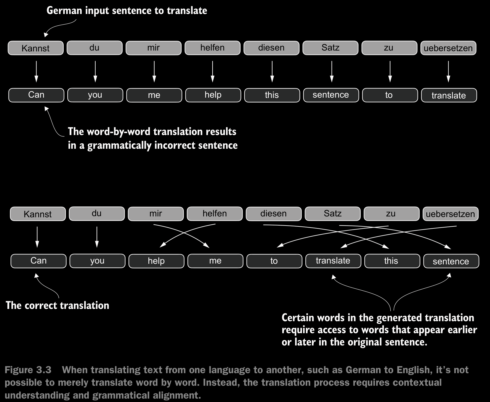
• To address this problem, it is common to use a deep neural network with two submodules, an encoder and a decoder. The job of the encoder is to first read in and process the entire text, and the decoder then produces the translated text.
• Before the advent of transformers, recurrent neural networks (RNNs) were the most popular encoder–decoder architecture for language translation. An RNN is a type of neural network where outputs from previous steps are fed as inputs to the current step, making them well-suited for sequential data like text.
• In an encoder–decoder RNN, the input text is fed into the encoder, which processes it sequentially. The encoder updates its hidden state (the internal values at the hidden layers) at each step, trying to capture the entire meaning of the input sentence in the final hidden state. The decoder then takes this final hidden state to start generating the translated sentence, one word at a time. It also updates its hidden state at each step, which is supposed to carry the context necessary for the next-word prediction.
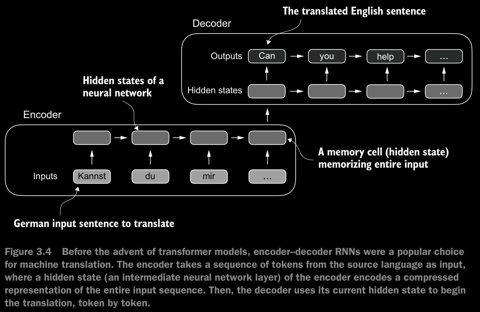
• The big limitation of encoder–decoder RNNs is that the RNN can’t directly access earlier hidden states from the encoder during the decoding phase. Consequently, it relies solely on the current hidden state, which encapsulates all relevant information. This can lead to a loss of context, especially in complex sentences where dependencies might span long distances.

3.2 Capturing Data Dependencies with Attention Mechanisms

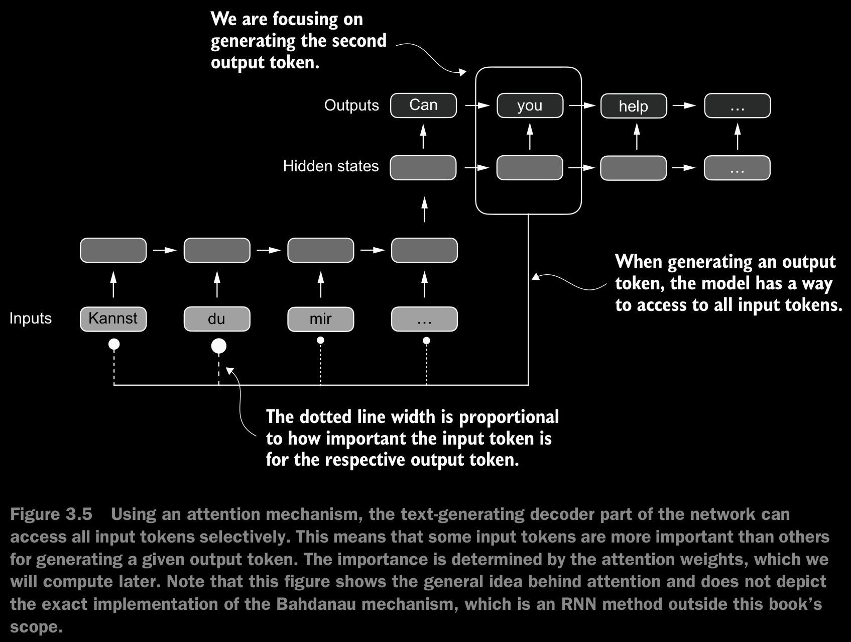
• Although RNNs work fine for translating short sentences, they don’t work well for longer texts as they don’t have direct access to previous words in the input. One majorshortcoming in this approach is that the RNN must remember the entire encoded input in a single hidden state before passing it to the decoder
• To solve this problem, researchers developed the Bahdanau attention mechanism for RNNs in 2014 (named after the first author of the respective paper B), which modifies the encoder-decoder RNN such that the decoder can selectively access different parts of the input sequence at each decoding step.
• Researchers found that RNN architectures are not required for building deep neural networks for natural language processing and proposed the original transformer architecture including a self-attention mechanism inspired by the Bahdanau attention mechanism.
• Self-attention is a mechanism that allows each position in the input sequence to consider the relevancy of, or “attend to,” all other positions in the same sequence when computing the representation of a sequence.

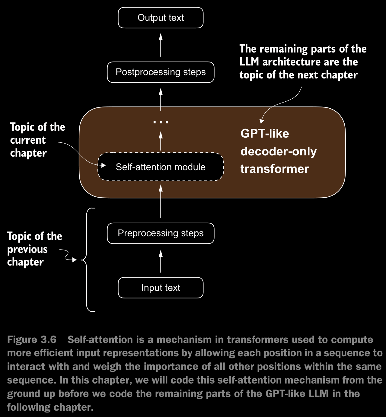
3.3 Attending to Different Parts of the Input with Self-Attention

• In self-attention, the “self” refers to the mechanism’s ability to compute attention weights by relating different positions within a single input sequence. It assesses and learns the relationships and dependencies between various parts of the input itself, such as words in a sentence or pixels in an image.
• This is in contrast to traditional attention mechanisms, where the focus is on the relationships between elements of two different sequences, such as in sequence-to-sequence models where the attention might be between an input sequence and an output sequence.

A simple Self-Attention Mechanism Without Trainable Weights

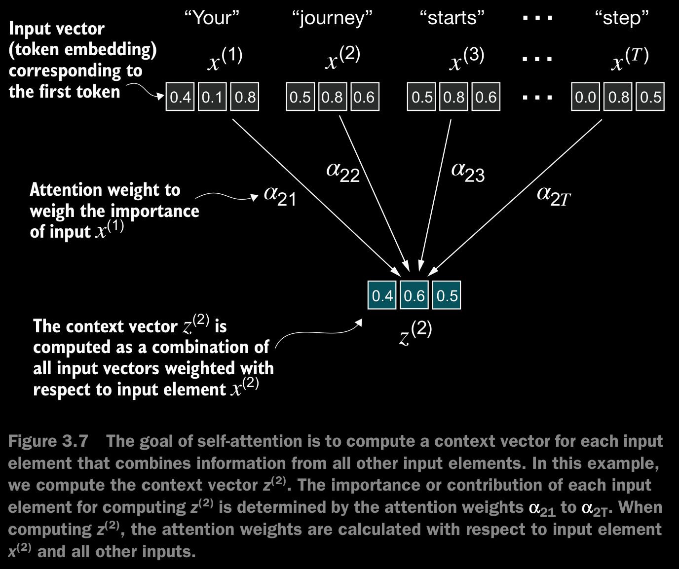
• Figure 3.7 shows an input sequence, denoted as $x$, consisting of $T$ elements represented as $x^{(1)}$ to $x^{(T)}$. This sequence typically represents text, such as a sentence, that has already been transformed into token embeddings.
• For example, consider an input text like “Your journey starts with one step”. In this case, each element of the sequence, such as $x^{(1)}$, corresponds to a $d$-dimensional embedding vector representing a specific token, like “Your.” Figure 3.7 shows these input vectors as 3-dimensional embeddings.
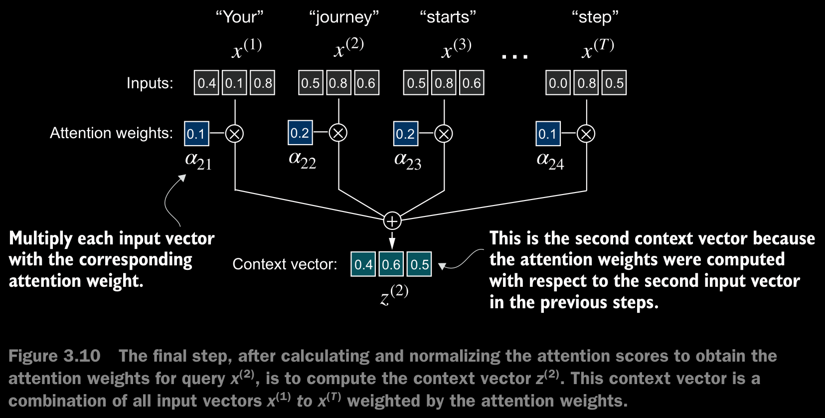
• In self-attention, our goal is to calculate context vectors $z^{(i)}$ for each element $x^{(i)}$ in the input sequence. A context vector can be interpreted as an enriched embedding vector.
• To illustrate this concept, let’s focus on the embedding vector of the second input element, $x^{(2)}$ (which corresponds to the token “journey”), and the corresponding context vector, $z^{(2)}$, shown at the bottom of figure 3.7. This enhanced context vector, $z^{(2)}$, is an embedding that contains information about $x^{(2)}$ and all other input elements, $x^{(1)}$ to $x^{(T)}$.
• Context vectors play a crucial role in self-attention. Their purpose is to create enriched representations of each element in an input sequence (like a sentence) by incorporating information from all other elements in the sequence (figure 3.7).
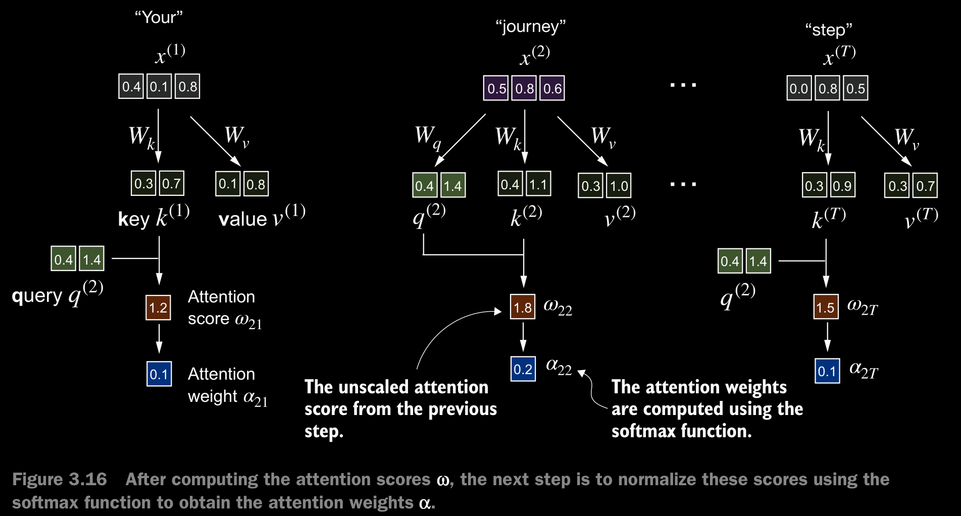
• The first step of implementing self-attention is to compute the intermediate values $\omega$, referred to as attention scores.
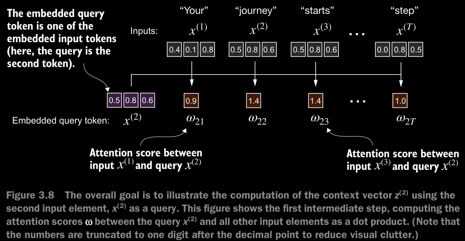
• We determine these scores by computing the dot product of the query, $x^{(2)}$, with every other input token.
• further implementation details in jupyter notebook
• In the context of self-attention mechanisms, the dot product determines the extent to which each element in a sequence focuses on, or “attends to,” any other element: the higher the dot product, the higher the similarity and attention score between two elements.
• we normalize each of the attention scores we computed previously. The main goal behind the normalization is to obtain attention weights that sum up to 1. This normalization is a convention that is useful for interpretation and maintaining training stability in an LLM.
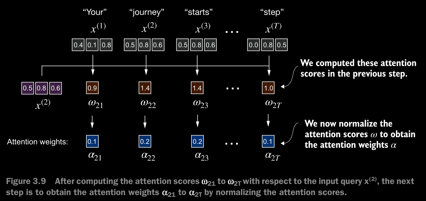
• In practice, it’s common and advisable to use the softmax function for normalization.
• The softmax function ensures that the attention weights are always positive apart from normalizing them. This makes the output interpretable as probabilities or relative importance, where higher weights indicate greater importance.
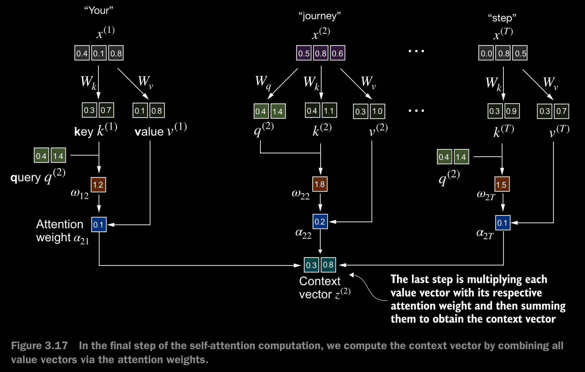
• Note that the naive softmax implementation torch.exp(x)/torch.exp(x).sum(dim=0) may encounter numerical instability problems, such as overflow and underflow, when dealing with large or small input values. Therefore, in practice, it’s advisable to use the PyTorch implementation of softmax, which has been extensively optimized and tested for performance.
• The context vector $z^{(2)}$ is calculated by multiplying the embedded input tokens, $x^{(i)}$, with the corresponding attention weights and then summing the resulting vectors. i.e., taking the wieghted sum of all input vectors, obtained by multiplying each input vector by its corresponding attention weight.

3.3.2 Computing Attention Weights for All Input Tokens

• Just expanding what is done above to all the elements.

attn_weights = torch.empty(inputs.shape[0], inputs.shape[0])
context_vects = torch.zeros(inputs.shape[0], inputs.shape[1])
 
for i, q_i in enumerate(inputs):
    for j, x_i in enumerate(inputs):
        attn_weights[i][j] = torch.dot(q_i, x_i)
 
attn_weights[i] = torch.softmax(attn_weights[i], dim=-1)
# By setting dim=-1, we are instructing the softmax function to apply the normalization along the last dimension of the attn_scores tensor
 
context_vects = attn_weights @ inputs # torch.matmul()
print(attn_weights)
print(context_vects)

3.4 Implementing Self-Attention With Trainable Weights

• This self-attention mechanism is also called scaled dot-product attention.
• The most notable difference from before is the introduction of weight matrices that are updated during model training. These trainable weight matrices are crucial so that the model (specifically, the attention module inside the model) can learn to produce “good” context vectors.

3.4.1 Computing the Attention Weights Step-by-Step

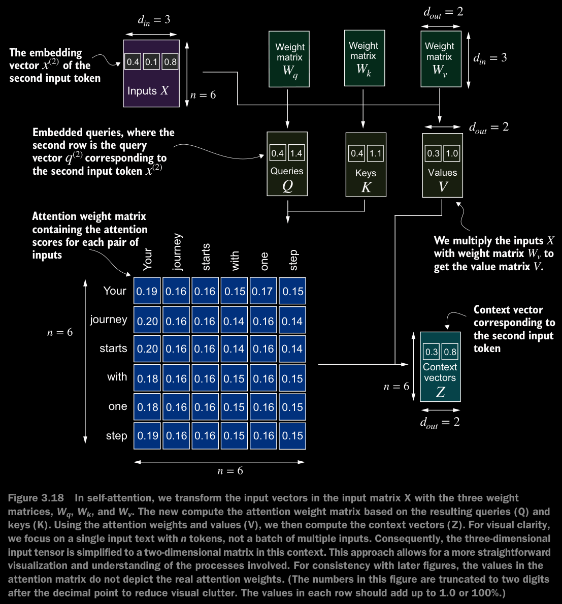
• We will implement the self-attention mechanism step by step by introducing the three trainable weight matrices $W_q$, $W_k$, and $W_v$. These three matrices are used to project the embedded input tokens, $x^{(i)}$, into query, key, and value vectors, respectively.
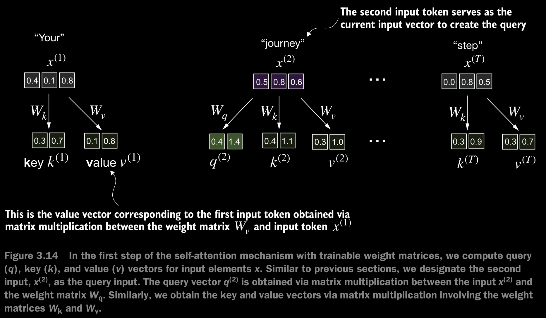
• We start here by computing only one context vector, $z^{(2)}$, for illustration purposes.
• Note that in GPT-like models, the input and output dimensions i.e., the dimentions of $W_{q/k/v}$ are usually the same.
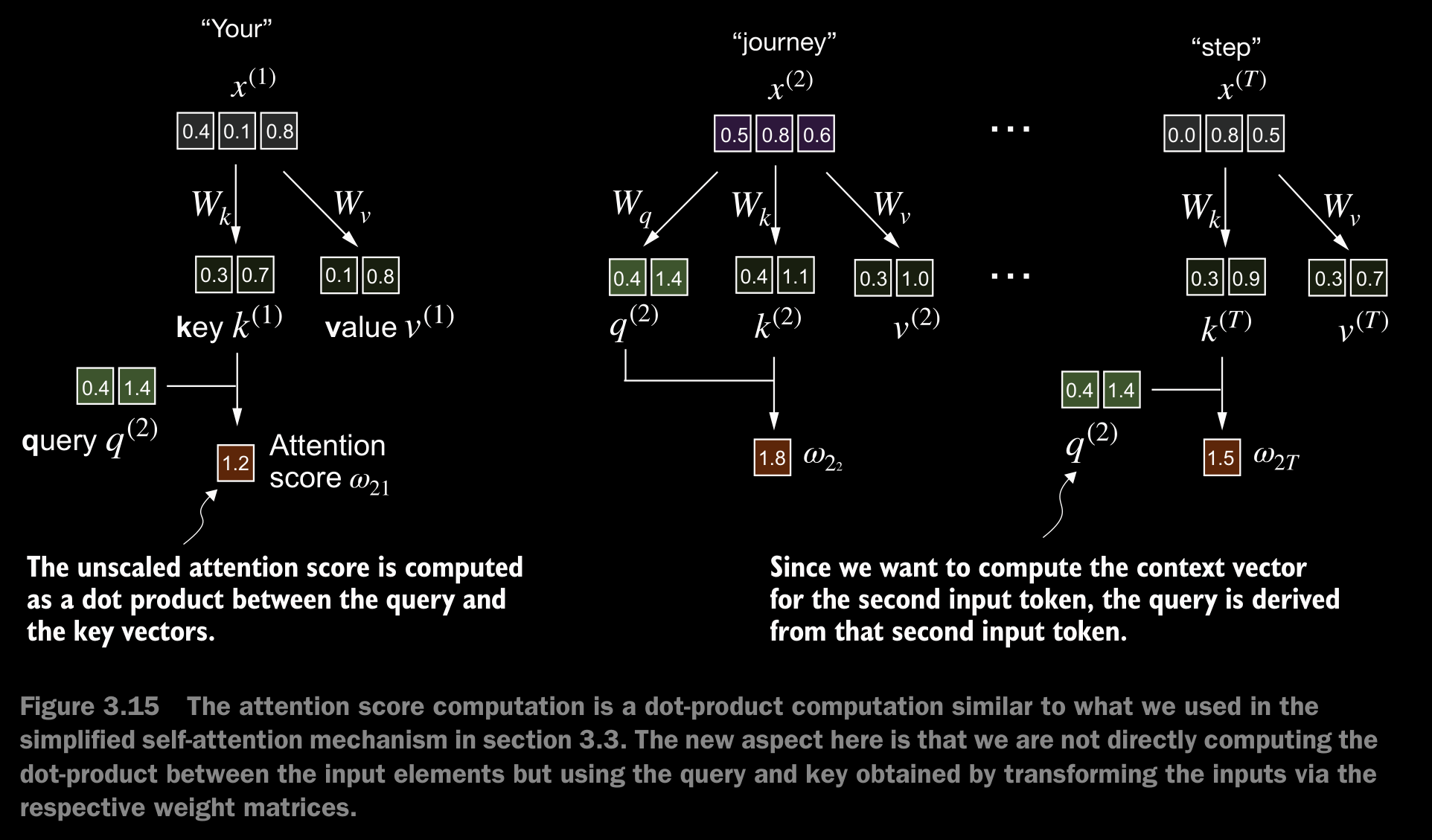
• Now, we want to go from the attention scores to the attention weights, as illustrated in figure 3.16. We compute the attention weights by scaling the attention scores and using the softmax function. However, now we scale the attention scores by dividing them by the square root of the embedding dimension of the keys (taking the square root is mathematically the same as exponentiating by 0.5).
• The reason for the normalization by the embedding dimension size is to improve the training performance by avoiding small gradients. For instance, when scaling up the embedding dimension, which is typically greater than 1,000 for GPT-like LLMs, large dot products can result in very small gradients during backpropagation due to the softmax function applied to them. As dot products increase, the softmax function behaves more like a step function, resulting in gradients nearing zero. These small gradients can drastically slow down learning or cause training to stagnate.
• The scaling by the square root of the embedding dimension is the reason why this self-attention mechanism is also called scaled-dot product attention.

Detailed Reasoning:

1. Why Scale by $\sqrt{d_k}$?

Without scaling, the dot product $Q{K}^T$ grows in magnitude with increasing $d_k$. Specifically, the dot product of two vectors $q$ and $k$ scales approximately with $d_k$ due to the summation of $d_k$ terms:

$$q\cdot k=\sum _{i=1}^{d_k}{q}_i{k}_i$$

If $q_i$ and $k_i$ are independent random variables with mean 0 and variance 1, the variance of the sum (i.e., $q\cdot k$) is proportional to $d_k$. Hence, the magnitude of the dot product increases with the embedding dimension $d_k$.

When $d_k$ is large (often $>1,000$ in GPT-like LLMs), the attention scores $Q{K}^T$ can become very large, leading to very high input values for the softmax function.

2. Effect of Large Dot Products on Softmax

The softmax function

$$\text{softmax}(x_i)=\frac{e^{x_i}}{{\sum }_j{e}^{x_j}}$$

transforms the attention scores into probabilities. When the values $x_i$ are large (because $Q{K}^T$ is large), the softmax behaves like a step function:

• Dominant Terms: The largest $x_i$ dominates the numerator $e^{x_i}$, making the corresponding softmax output close to 1.
• Non-Dominant Terms: All other terms in the denominator $e^{x_j}$ (for $j\ne i$) are comparatively small, making the corresponding softmax outputs close to 0.

As a result, the softmax outputs become highly saturated: one value is close to 1, while others are near 0.

3. Impact on Gradients

During backpropagation, the gradients of the loss function $L$ with respect to the attention scores $z_i$ (i.e., $\frac{\partial L}{\partial z_i}$) are influenced by the derivative of the softmax function:

$$\frac{\partial \text{softmax}(x_i)}{\partial x_j}=\text{softmax}(x_i)({\delta }_{ij}-\text{softmax}(x_j))$$

When the softmax outputs are close to 1 and 0 (due to large dot products), the derivatives become very small:

• If $\text{softmax}(x_i)\approx 1$, then $\text{softmax}(x_i)(1-\text{softmax}(x_i))\approx 0$.
• If $\text{softmax}(x_i)\approx 0$, then $\text{softmax}(x_i)(1-\text{softmax}(x_i))\approx 0$.

These small derivatives (gradients) propagate back through the network, resulting in vanishing gradients. When gradients vanish, the model updates are very small, slowing down learning or causing training to stagnate.

4. Normalization by $\sqrt{d_k}$

To counteract the effect of large dot products, we scale the attention scores by $\frac{1}{\sqrt{d_k}}$ before applying the softmax:

$$\frac{Q{K}^T}{\sqrt{d_k}}$$

This scaling reduces the magnitude of the dot products, ensuring that the inputs to the softmax remain within a reasonable range. Consequently:

• The attention scores are less extreme, avoiding saturation in the softmax outputs.
• The gradients $\frac{\partial L}{\partial z_i}$ remain sufficiently large, allowing effective backpropagation and preventing vanishing gradients.

---

• Next step is to calculate the Context Vector $z^{(2)}$

Why query, key, and value?

• The terms “key,” “query,” and “value” in the context of attention mechanisms are borrowed from the domain of information retrieval and databases, where similar concepts are used to store, search, and retrieve information.
• A query is analogous to a search query in a database. It represents the current item (e.g., a word or token in a sentence) the model focuses on or tries to understand. The query is used to probe the other parts of the input sequence to determine how much attention to pay to them.
• The key is like a database key used for indexing and searching. In the attention mechanism, each item in the input sequence (e.g., each word in a sentence) has an associated key. These keys are used to match the query.
• The value in this context is similar to the value in a key-value pair in a database. It represents the actual content or representation of the input items. Once the model determines which keys (and thus which parts of the input) are most relevant to the query (the current focus item), it retrieves the corresponding values.

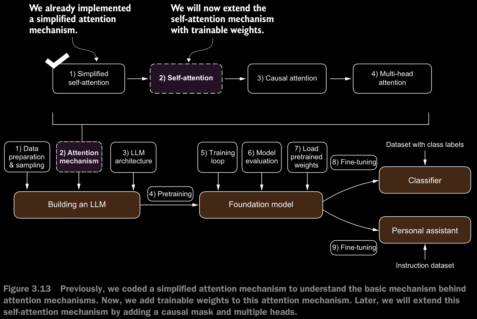
3.4.2 Implementing a Compact Self-Attention Python Class

$$\mathrm{Attention}(Q,K,V)=\mathrm{softmax}\left(\frac{Q{K}^T}{\sqrt{d_k}}\right)V$$

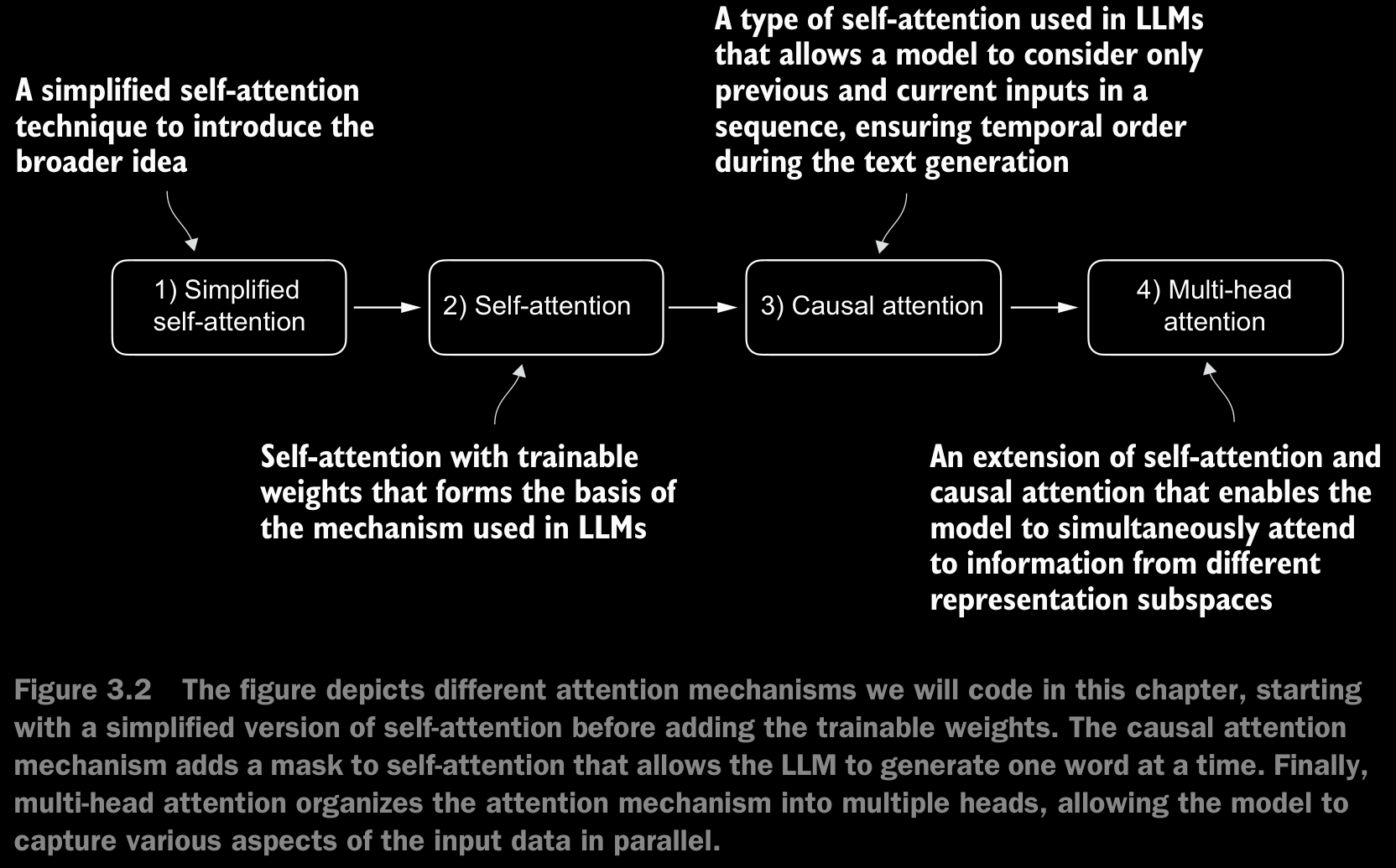
• Next, we will make enhancements to the self-attention mechanism, focusing specifically on incorporating causal and multi-head elements.
• The causal aspect involves modifying the attention mechanism to prevent the model from accessing future information in the sequence, which is crucial for tasks like language modeling, where each word prediction should only depend on previous words.

3.5 Hiding Future Words with Causal Attention

• Causal attention, also known as masked attention, is a specialized form of self-attention. It restricts a model to only consider previous and current inputs in a sequence when processing any given token when computing attention scores. This is in contrast to the standard self-attention mechanism, which allows access to the entire input sequence at once.
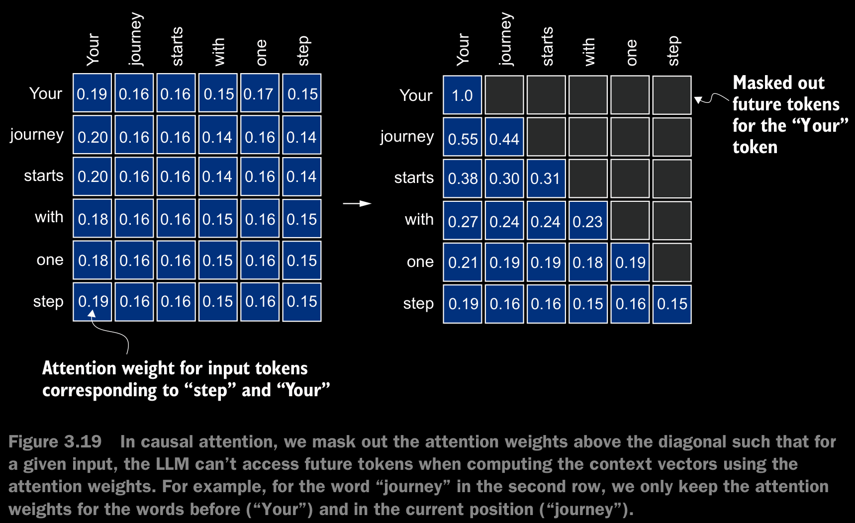
• We mask out the attention weights above the diagonal, and we normalize the nonmasked attention weights such that the attention weights sum to 1 in each row.

3.5.1 Applying a Causal Attention Mask

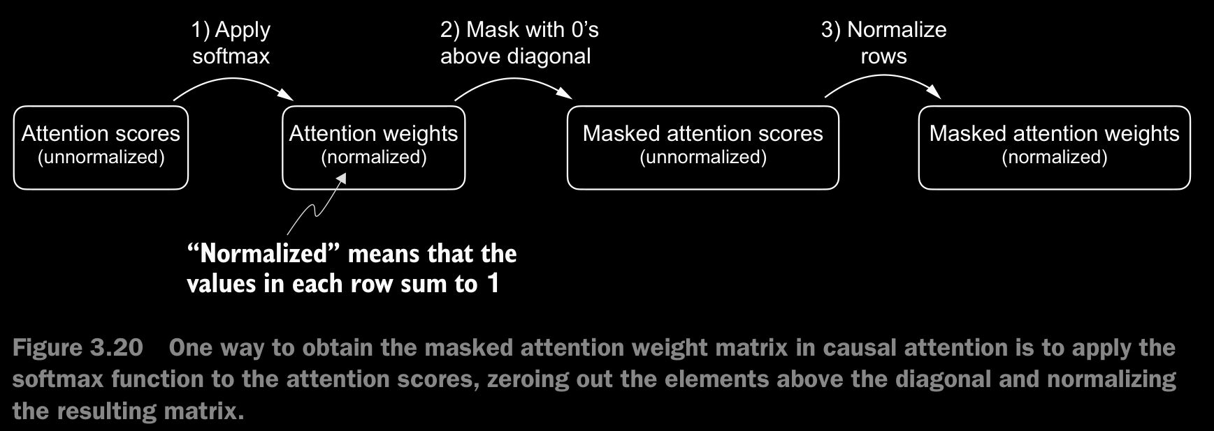
• For the renormalization after masking, We divide each element in each row by the sum in each row.
• When we apply a mask and then renormalize the attention weights, it might initially appear that information from future tokens (which we intend to mask) could still influence the current token because their values are part of the softmax calculation. However, the key insight is that when we renormalize the attention weights after masking, what we’re essentially doing is recalculating the softmax over a smaller subset (since masked positions don’t contribute to the softmax value). The mathematical elegance of softmax is that despite initially including all positions in the denominator, after masking and renormalizing, the effect of the masked positions is nullified—they don’t contribute to the softmax score in any meaningful way. In simpler terms, after masking and renormalization, the distribution of attention weights is as if it was calculated only among the unmasked positions to begin with. This ensures there’s no information leakage from future (or otherwise masked) tokens as we intended.
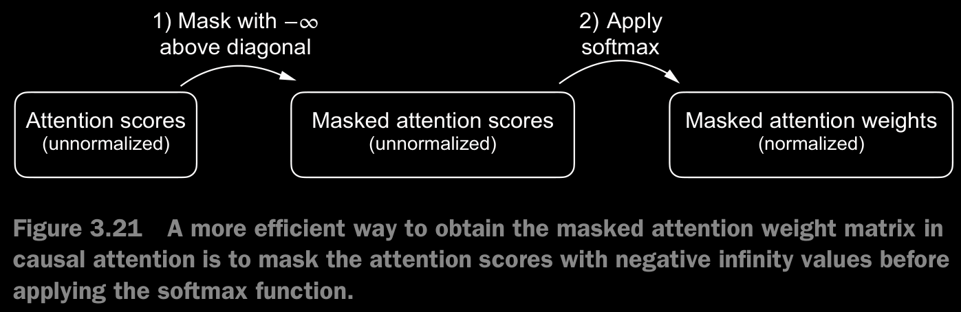
• The better method for making the attention causal is to set the non-lower-trainagular matrix part to $-\infty$ in the attention scores matrix. When softmax is applied, all the $-\infty$ terms convert to $\approx 0$ terms. If done this way, there is no need for renormalization and the efficiency is improved.

3.5.2 Masking Additional Attention Weights With Dropout

• Dropout in deep learning is a technique where randomly selected hidden layer units are ignored during training, effectively “dropping” them out. This method helps prevent overfitting by ensuring that a model does not become overly reliant on any specific set of hidden layer units.
• In the transformer architecture, including models like GPT, dropout in the attention mechanism is typically applied at two specific times:
  • after calculating the attention weights or
  • after applying the attention weights to the value vectors i.e., after calculating context vectors.
• Here we will apply the dropout mask after computing the attention weights.
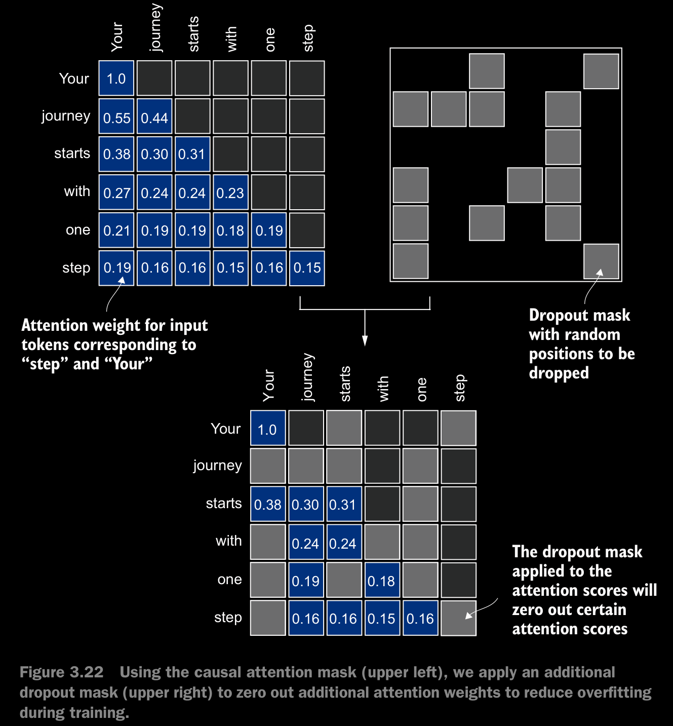
• To compensate for the reduction in active elements, the values of the remaining elements in the matrix are scaled up by a factor of $1/p$ (done by pytorch’s nn.Dropout automatically). This scaling is crucial to maintain the overall balance of the attention weights, ensuring that the average influence of the attention mechanism remains consistent during both the training and inference phases.

3.5.3 Implementing a Compact Causal Attention Class

• This class will then serve as a template for developing multi-head attention, which is the final attention class we will implement.
• First we have to make sure that the code can handle batches consisting of more than one input so that the CausalAttention class supports the batch outputs produced by the data loader we implemented in chapter 2.
• about register_buffer() method used in the code implementation register_buffer()

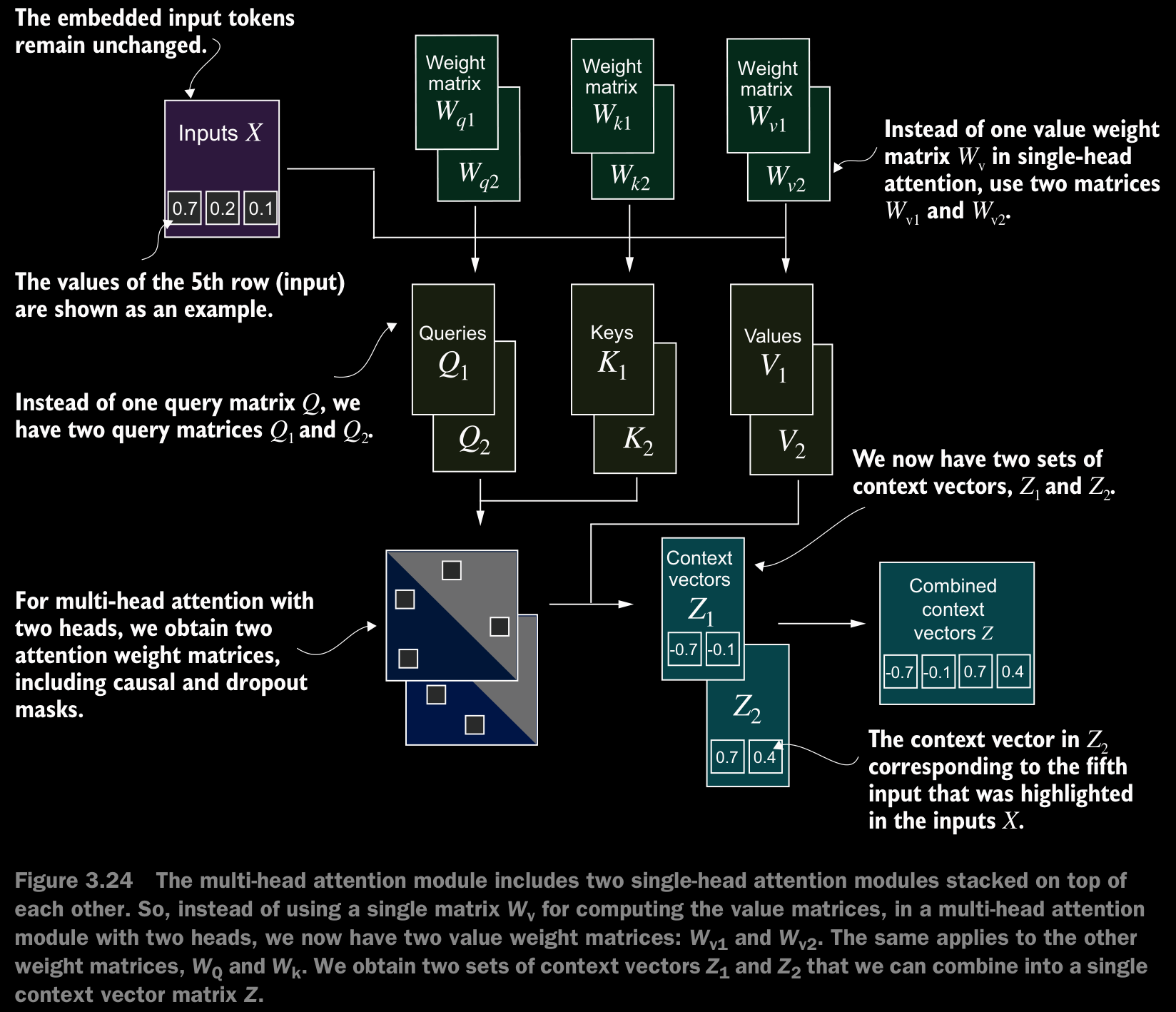
3.6 Extending Single-Head Attention to Multi-Head Attention

• Our final step will be to extend the previously implemented causal attention class over multiple heads. This is also called multi-head attention.
• The term “multi-head” refers to dividing the attention mechanism into multiple “heads,” each operating independently. In this context, a single causal attention module can be considered single-head attention, where there is only one set of attention weights processing the input sequentially.

3.6.1 Stacking Multiple Single-Head Attention Layers

• In practical terms, implementing multi-head attention involves creating multiple instances of the self-attention mechanism, each with its own weights, and then combining their outputs.
• Using multiple instances of the self-attention mechanism can be computationally intensive, but it’s crucial for the kind of complex pattern recognition that models like transformer-based LLMs are known for.
• The main idea behind multi-head attention is to run the attention mechanism multiple times (in parallel) with different, learned linear projections—the results of multiplying the input data (like the query, key, and value vectors in attention mechanisms) by a weight matrix. In code, we can achieve this by implementing a simple MultiHeadAttentionWrapper class that stacks multiple instances of our previously implemented CausalAttention module.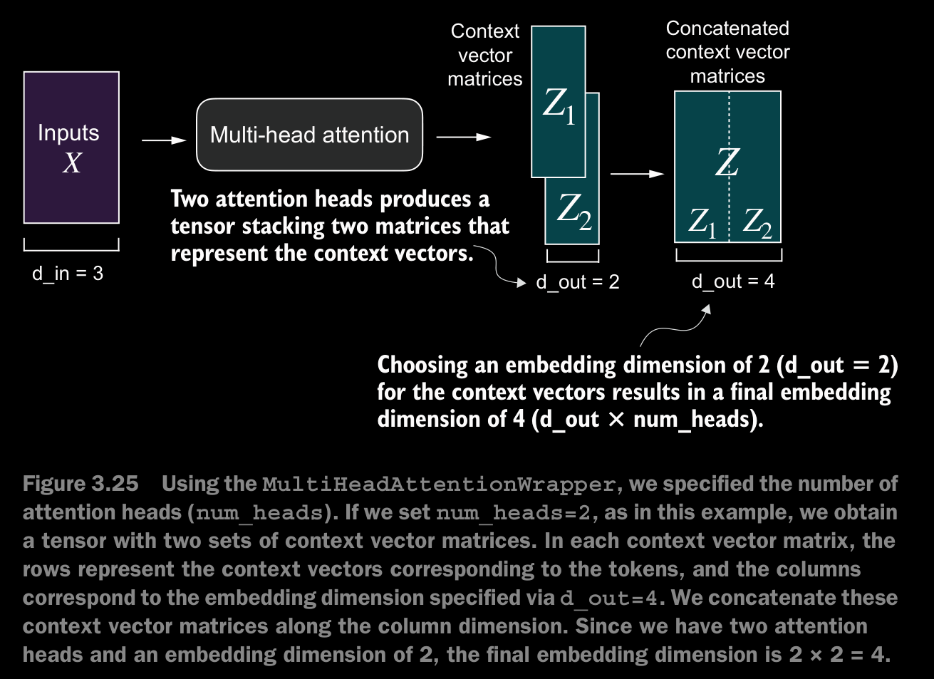

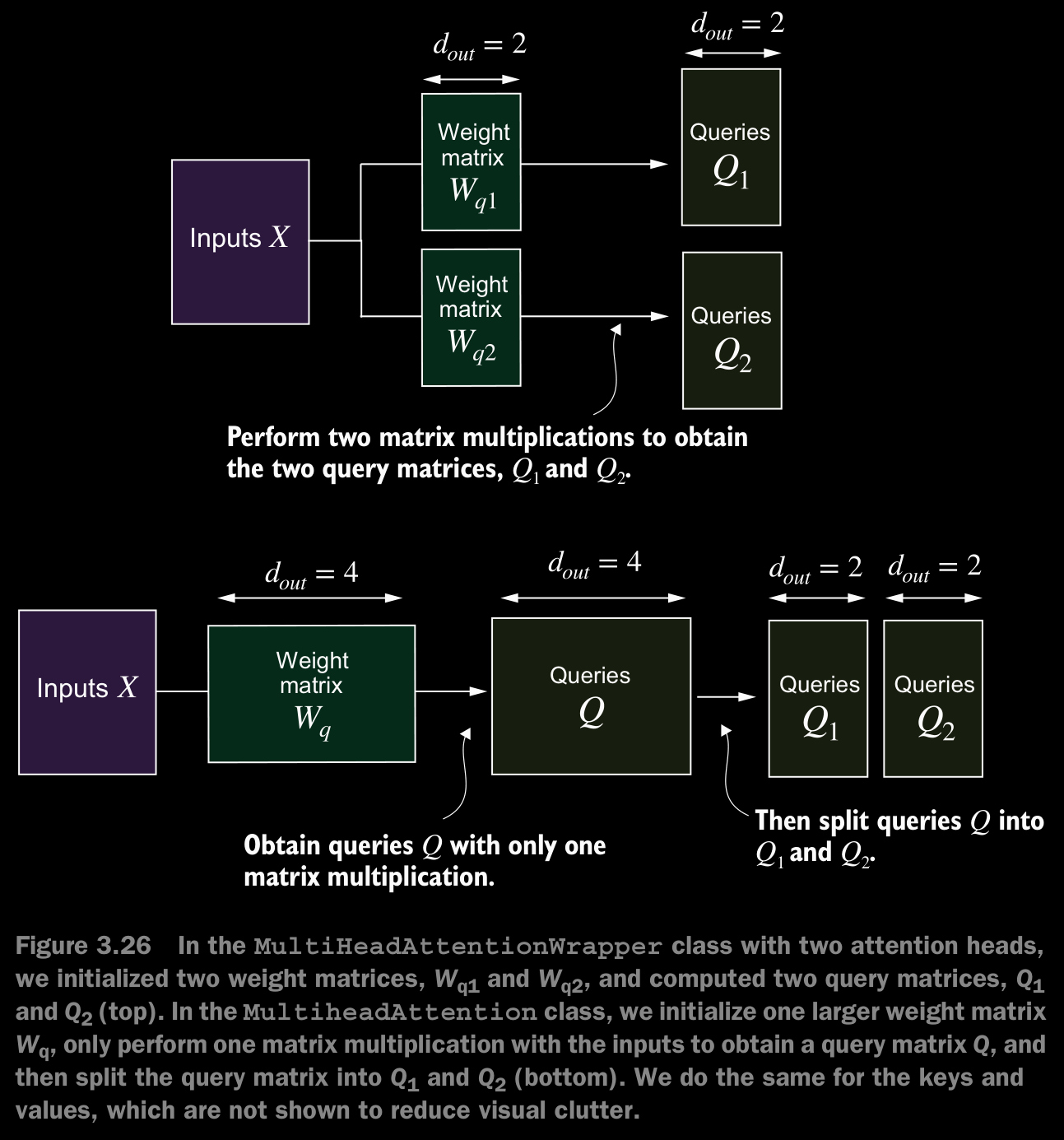
3.6.2 Implementing Multi-Head Attention With Weight Splits

• Instead of maintaining two separate classes, MultiHeadAttentionWrapper and CausalAttention, we can combine these concepts into a single MultiHeadAttention class. Also, in addition to merging the MultiHeadAttentionWrapper with the CausalAttention code, we will make some other modifications to implement multi-head attention more efficiently.
• This class splits the input into multiple heads by reshaping the projected query, key, and value tensors and then combines the results from these heads after computing attention.
• In the implementaion, we added an output projection layer (self.out_proj) to MultiHeadAttention after combining the heads, which is not present in the CausalAttention class. This output projection layer is not strictly necessary, but it is commonly used in many LLM architectures, which is why it is added here for completeness.
• Even though the MultiHeadAttention class looks more complicated than the MultiHeadAttentionWrapper due to the additional reshaping and transposition of tensors, it is more efficient.
• In the MultiHeadAttentionWrapper, we needed to repeat the matrix multiplications, which is computationally one of the most expensive steps, for each attention head.
• The embedding sizes of the token inputs and context embeddings are the same in GPT models (d_in = d_out).