ResNet - Deep Residual Learning for Image Recognition

1. Introduction

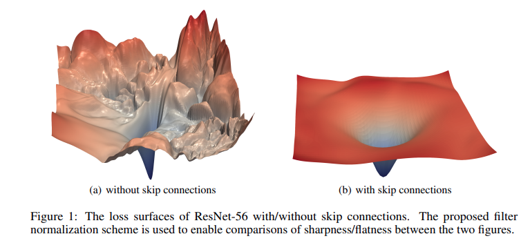
When deeper networks are able to start converging, a degradation problem has been exposed: with the network depth increasing, accuracy gets saturated (which might be unsurprising) and then degrades rapidly. Unexpectedly, such degradation is not caused by overfitting, and adding more layers to a suitably deep model leads to higher training error, as reported in [11, 42] and thoroughly verified by our experiments. Fig. 1 shows a typical example.

source

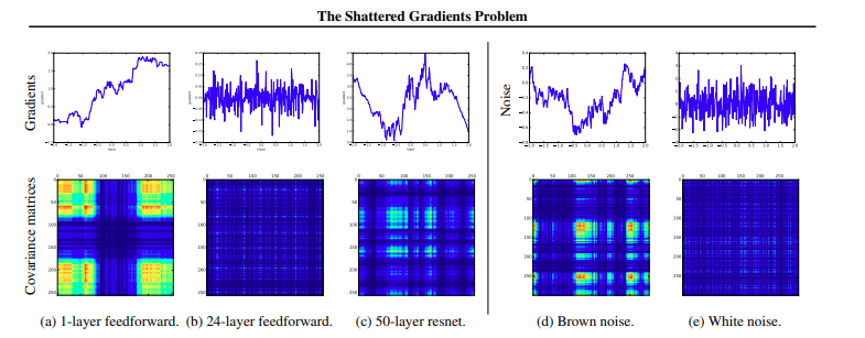
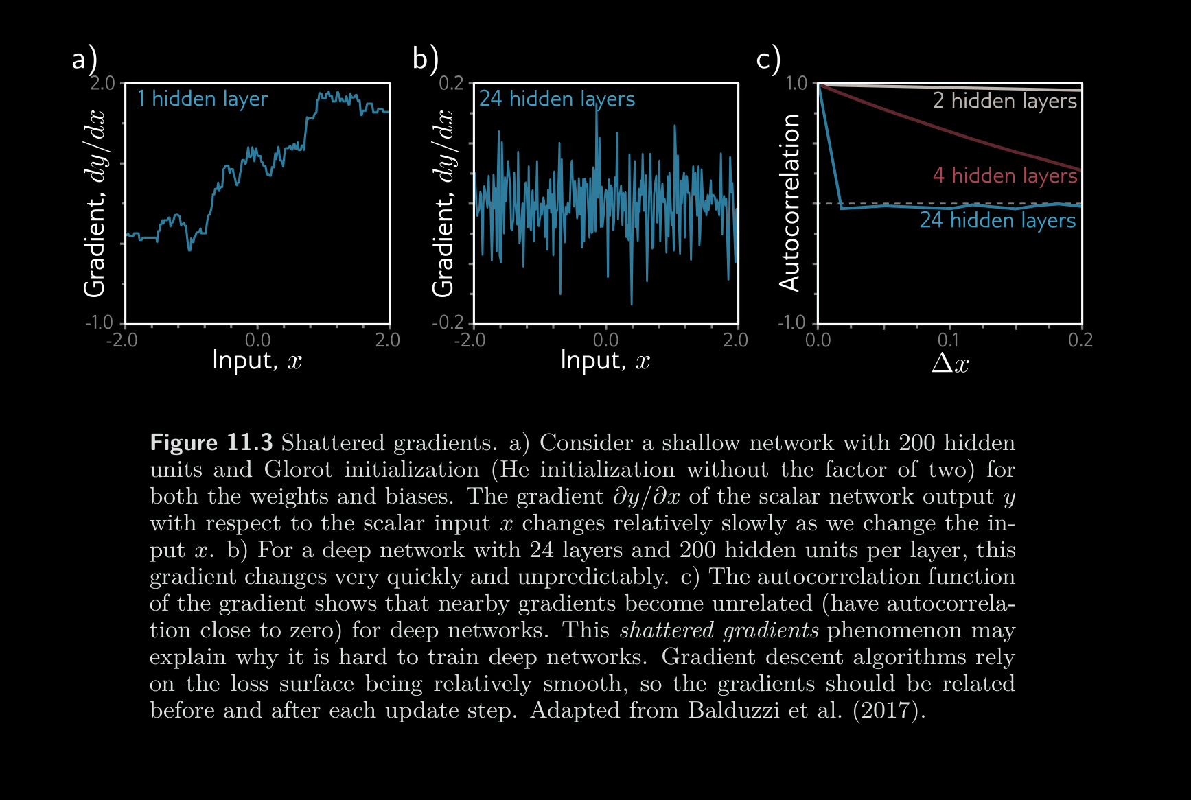
This phenomenon is not completely understood. One conjecture is that at initialization, the loss gradients change unpredictably when we modify parameters in early network layers. With appropriate initialization of the weights (see section 7.5), the gradient of the loss with respect to these parameters will be reasonable (i.e., no exploding or vanishing gradients). However, the derivative assumes an infinitesimal change in the parameter, whereas optimization algorithms use a finite step size. Any reasonable choice of step size may move to a place with a completely different and unrelated gradient; the loss surface looks like an enormous range of tiny mountains rather than a single smooth structure that is easy to descend. Consequently, the algorithm doesn’t make progress in the way that it does when the loss function gradient changes more slowly. This conjecture is supported by empirical observations of gradients in networks with a single input and output. For a shallow network, the gradient of the output with respect to the input changes slowly as we change the input (figure 11.3a). However, for a Autocorrelation function deep network, a tiny change in the input results in a completely different gradient (figure 11.3b). This is captured by the autocorrelation function of the gradient (figure 11.3c). Nearby gradients are correlated for shallow networks, but this correlation quickly drops to zero for deep networks. This is termed the shattered gradients phenomenon.

source: Understanding Deep Learning pg.187, 11.1.1 Limitations of sequential processing

source: Understanding Deep Learning pg.187, 11.1.1 Limitations of sequential processing Autocorrelation

The phenomenon of shattered gradients arises due to the increasing complexity of how changes in early network layers influence the output as the network depth increases. Specifically, the derivative of the output $y$ with respect to the first layer $f_{1}$ of the network is given by:

\frac{\partial y}{\partial f _{1}} = \frac{\partial f _{2}}{\partial f _{1}} \cdot \frac{\partial f _{3}}{\partial f _{2}} \cdot \frac{\partial f _{4}}{\partial f _{3}} \dots

When we alter the parameters governing $f_{1}$ , each derivative in this sequence is evaluated at slightly different points, as layers $f_{2}$ , $f_{3}$ , and $f_{4}$ are all derived from $f_{1}$ .

As a result, the updated gradient for each training example may vary significantly, leading to instability in the loss function’s behavior, often referred to as a “badly behaved” loss landscape. This can make training deep networks challenging as gradients may lose coherence and diminish, hence the term “shattered gradients.”

3. Deep Residual Learning

3.1 Residual Learning

To handle cases where the dimensions of $x$ and $F (x, {W_{i}})$ do not match, we introduce a linear projection $W_{s}$ applied to $x$ to transform it to the same dimensions as $F (x, {W_{i}})$ . This projection is typically implemented using a 1x1 convolutional layer, which changes the number of channels in $x$ without affecting its spatial dimensions. The updated residual block equation becomes:

y = F (x, {W_{i}}) + W_{s} x

Here:

$W_{s}$ is the projection that aligns the dimensions of $x w i t h$ F(x, {W_i})$.
This ensures that the addition $F (x, {W_{i}}) + W_{s} x$ is valid because both terms now have the same dimensions.

Code

def forward(self, x):
	residual = x
	# applying a downsample function before adding it to the output
	if(self.downsample is not None):
		residual = downsample(residual)
 
	out = F.relu(self.bn(self.conv1(x)))
 
	out = self.bn(self.conv2(out))
	# note that adding residual before activation
	out = out + residual
	out = F.relu(out)
	return out

The original paper uses strided convolutions to downsample the image. The main path is downsampled automatically using these strided convolutions as is done normally in code. The residual path uses either (a) identity mapping with zero entries added to add no additional parameters or (b) a 1x1 convolution with the same stride parameter.

The second option could look like follows:

if downsample:
    self.downsample = conv1x1(inplanes, planes, strides

Exploding Gradients

Adding residual connections roughly doubles the depth of a network that can be practically trained before performance degrades. We can’t increase the depth arbritrarity because of exploding gradients and forward activation values.

In deep neural networks, especially residual networks (ResNets), exploding gradients and forward activation values pose significant challenges during training.

1. Importance of Proper Initialization

When training deep networks, careful initialization of network parameters is critical for stability. Without it, values in the network can either grow or shrink exponentially, leading to two main issues:

Exploding values: This occurs when the values in the network increase exponentially as we move through layers.
Vanishing values: Conversely, values can diminish to near zero across layers.

These issues arise in both:

Forward Pass: During the forward pass, if intermediate activations grow exponentially, they may exceed numerical precision, leading to errors.
Backward Pass: During backpropagation, gradients can explode (grow too large) or vanish (become nearly zero), which severely hampers learning.

To counteract these effects, initializations like He initialization are used for networks with ReLU activations. This initialization:

Sets biases ( $β$ ) to zero.
Chooses weights ( $Ω$ ) from a normal distribution with mean zero and variance $\frac{2}{D _{h}}$ , where $D_{h}$ is the number of hidden units in the previous layer.
Ensures that, on average, the activations and gradients maintain the same variance between layers, thus helping to stabilize both forward and backward passes.

2. Vanishing Gradients in Residual Networks

Residual networks are designed to allow information to flow easily across layers by introducing skip (or shortcut) connections. These connections provide a direct path for the data to travel from one layer to another without additional transformations.

In a ResNet:

Each layer contributes directly to the final output, providing alternative paths for gradients during backpropagation, which mitigates the vanishing gradient problem.
Even if certain gradients diminish in deeper layers, other gradients still pass through the skip connections, improving gradient flow and enabling deeper architectures.

3. Problem of Variance Doubling in Residual Blocks

Even though skip connections solve the vanishing gradient problem, they introduce a new issue in ResNets: exploding gradients due to variance doubling. Here’s how this happens:

Structure of Residual Block: In each residual block, the output of some processing layer (e.g., nonlinear transformations, convolutions) is added back to the input of that block. This operation is the key feature of the residual network.
Variance Growth: Each residual block introduces some variance in the activations. When we add the output of the block back to the input, the variance of the combined output doubles.
- For example, let’s assume the variance of the input is $σ^{2}$ , and the variance of the residual block’s output is also $σ^{2}$ (as He initialization helps keep the variance stable within the block). When they are combined through addition, the total variance becomes $2 σ^{2}$ .
- With each added residual block, this variance grows exponentially with depth, doubling with each layer. Thus, the deeper the ResNet, the greater the risk of having extremely large activations and gradients, which can lead to instability in training.

4. Stabilization Techniques

To address this variance growth, we can use the following techniques:

Scaling the Residual Block Output: One approach is to multiply the output of each residual block by $\frac{1}{2}$ before adding it back to the input. This scaling compensates for the doubling effect, keeping the variance stable as we move deeper into the network. Mathematically, this ensures that the variance remains close to the original $σ^{2}$ value across layers rather than doubling each time.
Batch Normalization: Batch normalization is the most common solution used in practice. Batch normalization:
- Normalizes the output of each layer to have a consistent mean and variance.
- Prevents variance from growing exponentially as we go deeper in the network by constraining values to a certain range.
- Is applied to each residual block’s output, making it robust to exploding or vanishing values, and thus stabilizing both the forward and backward passes.

Here’s a breakdown of the key concepts in Batch Normalization (BatchNorm), specifically how it’s applied in neural networks, including residual networks.

5. How Batch Normalization Works

BatchNorm operates by shifting and rescaling the activations, $h$ , to match desired statistical properties, specifically mean and variance. The process follows these steps:

Step 1: Compute Batch Statistics

For a given batch $B$ of activations $h$ :

Mean, $m_{h}$ : Compute the average of the activations across the batch: $m_{h} = \frac{1}{∣ B ∣} i \in B \sum h_{i}$
Standard Deviation, $s_{h}$ : Calculate the standard deviation to capture the spread of activations: $s_{h} = \frac{1}{∣ B ∣} i \in B \sum (h_{i} - m_{h})^{2}$

Step 2: Standardize Activations

Each activation $h_{i}$ in the batch is then standardized:

h_{i} \leftarrow \frac{h _{i} - m _{h}}{s _{h} + ϵ}

where $ϵ$ is a small constant added to prevent division by zero. After this step, the activations have a mean of zero and a unit variance.

Step 3: Scale and Shift

To allow the model to learn optimal scaling and shifting for each normalized activation, BatchNorm introduces two new parameters:

Scale $γ$ : Controls the variance of the activations.
Shift $δ$ : Controls the mean of the activations.

The standardized activation $h_{i}$ is then transformed as:

h_{i} \leftarrow γ h_{i} + δ

After this operation, the activations across the batch have a mean of $δ$ and a standard deviation of $γ$ , allowing the model to adjust these values during training.

6. Impact on Residual Networks

In residual networks:

Variance Control: BatchNorm helps prevent the exponential variance growth that occurs from adding residuals to inputs, as each block’s variance doubles without normalization.
Initialization: In each residual block, BatchNorm is often applied as the first step, with the initial $δ = 0$ and $γ = 1$ . Combined with He initialization, this stabilizes the variance at each layer, reducing the likelihood of exploding or vanishing gradients.
Identity Approximation: At initialization, layers with BatchNorm in residual networks tend to approximate the identity function because the residual connection dominates the output. This allows residual networks to be extremely deep without destabilizing training.

7. BatchNorm in Training vs. Inference

Training Mode: During training, the batch mean $m_{h}$ and standard deviation $s_{h}$ are recalculated for each batch.
Inference Mode: At test time, a batch isn’t available to calculate these statistics. Instead, global statistics (mean and variance) are calculated over the entire training dataset and “frozen” to ensure consistent behavior during inference.

After this, read Identity Mappings in Deep Residual Networks

🤓 Yashwanth's Notes

Explorer