4. Implementing a GPT Model From Scratch to Generate Text

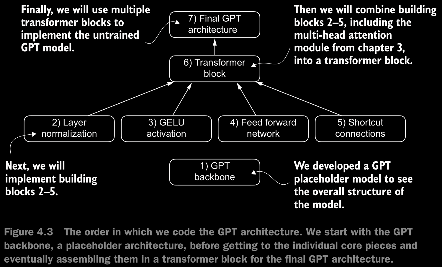
4.1 Coding an LLM Architecture

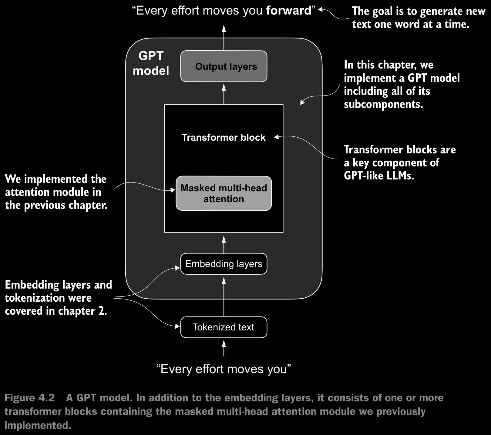
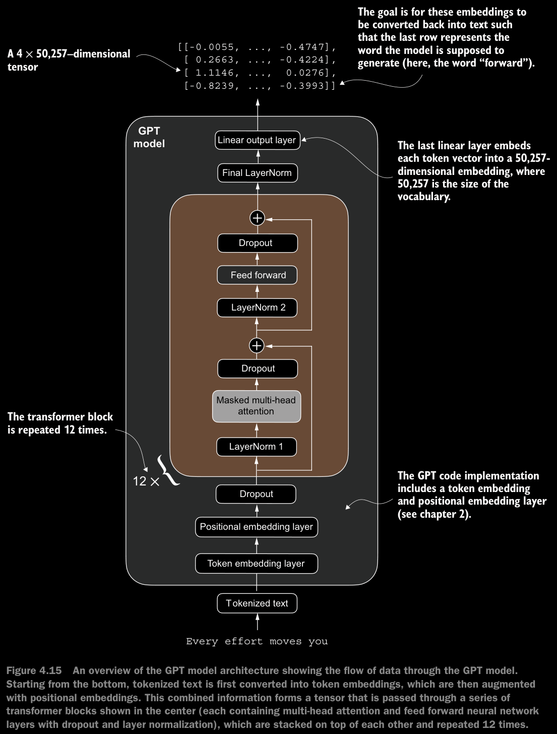
• Data flow through the model:
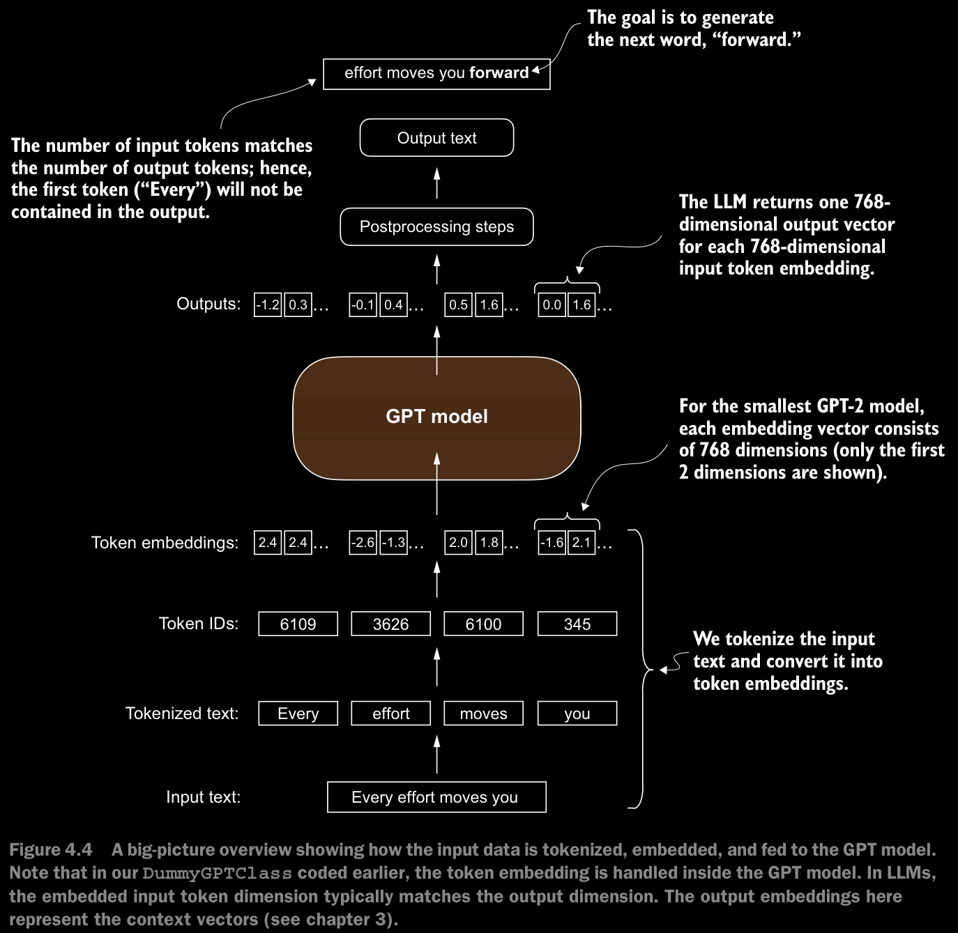
  1. compute token embeddings
  2. compute positional embeddings
  3. combine to get final embeddings
  4. apply dropout on the embeddings
  5. pass them through the transformer blocks
  6. do a layer normalization on the output
  7. pass it through the final linear layer to get the ouput logits
• Here, dropout is applied ot the token embeddings before passing them through the transformer blocks. This is to regularize the model at the input level. Transformers, especially the large ones, can memorize the patterns in data very easily. This is especially important for long sequences where the likelyhood of a token dominating the attention is high. This also helps in reducing the over-reliance which might occur on the positional embeddings.
• The purpose of out_head in the DummyGPTModel is to map the final hidden states to the vocabulary space, generating logits for each token prediction.

4.2 Normalizing Activations WIth Layer Normalization

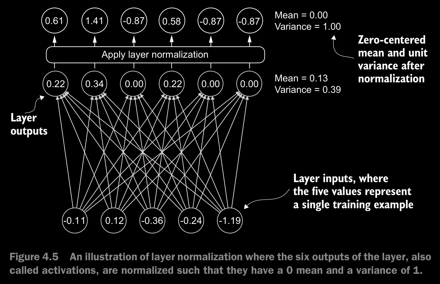
• The main idea behind layer normalization is to adjust the activations (outputs) of a neural network layer to have a mean of 0 and a variance of 1, also known as unit variance. This adjustment speeds up the convergence to effective weights and ensures consistent, reliable training.
• In GPT-2 and modern transformer architectures, layer normalization is typically applied before and after the multi-head attention module, and before the final output layer.
• The scale and shift are two trainable parameters (of the same dimension as the input) that the LLM automatically adjusts during training if it is determined that doing so would improve the model’s performance on its training task. This allows the model to learn appropriate scaling and shifting that best suit the data it is processing.
• This specific implementation of layer normalization operates on the last dimension of the input tensor x, which represents the embedding dimension (emb_dim).

1. Variance Calculation Basics

Population vs. Sample Variance

Variance is a measure of how much a set of numbers deviates from the mean. There are two primary types of variance:

1. Population Variance (biased):
   • When you calculate the variance for an entire population (all possible data points), the formula is:

$${\sigma }^2=\frac{1}{n}\sum _{i=1}^n(x_i-\mu {)}^2$$

• Where:
  • $n$ = the total number of data points
  • $x_i$ = each individual data point
  • $\mu$ = the mean of the data points

2. Sample Variance (unbiased):
   • When you calculate the variance from a sample (a subset of the population), the formula typically uses Bessel’s correction, where you divide by $n-1$ instead of $n$:

$$\frac{1}{n-1}\sum _{i=1}^n(x_i-\bar{x}{)}^2$$

• Where:
  • $\bar{x}$ = the sample mean

Why Use $n-1$ for Sample Variance?

• When calculating the variance from a sample, using $n-1$ helps correct for the fact that the sample mean $\bar{x}$ tends to be closer to the sample data points than the true population mean $\mu$.
• This correction accounts for the fact that samples inherently underestimate the variability in the full population.
• The $n-1$ divisor makes the estimate unbiased, meaning it more accurately reflects the true population variance when averaged over many samples.

2. Biased vs. Unbiased Variance in Practice

When is Each Method Used?

1. Biased Variance (dividing by $n$):
   • Commonly used when you have the full dataset or when you don’t need to correct for bias.
   • Often used in machine learning and deep learning contexts, especially when the dataset is large or when normalization layers are involved.
2. Unbiased Variance (dividing by $n-1$):
   • Used when estimating the variance of a population from a small sample.
   • More appropriate for statistical analysis where accuracy in estimating the true population variance is critical.

In Code (e.g., PyTorch or NumPy):

• In libraries like PyTorch and NumPy, the parameter unbiased determines whether to apply Bessel’s correction:

torch.var(tensor, unbiased=True)    # Unbiased variance (uses n - 1)
torch.var(tensor, unbiased=False)   # Biased variance (uses n)

3. Why Use Biased Variance in LLMs?

1. Large Embedding Dimensions:
   • LLMs, like GPT-2, operate in very high-dimensional spaces where the embedding dimension $n$ can be in the thousands or tens of thousands.
   • When $n$ is very large, the difference between $n$ and $n-1$ becomes negligible:

$$\frac{1}{n}\approx \frac{1}{n-1}\text{for large }n$$

2. Compatibility with GPT-2:
   • GPT-2’s original implementation (in TensorFlow) uses the biased variance calculation by default.
   • To ensure compatibility with pretrained weights and normalization layers in GPT-2, it’s important to follow the same variance calculation method.
   • Consistency in normalization layers helps maintain the model’s performance and avoids discrepancies during training or inference.

4. Normalization Layers in LLMs

In transformer models like GPT-2, Layer Normalization is used extensively to stabilize training. It normalizes the inputs to a layer so that they have a consistent mean and variance. The normalization formula typically looks like:

$$\text{LayerNorm}(x)=\frac{x-\mu }{\sqrt{{\sigma }^2+ϵ}}$$

Where:

• $\mu$ = mean of the inputs
• ${\sigma }^2$ = variance of the inputs (calculated as biased in this context)
• $ϵ$ = a small constant for numerical stability Using a biased variance (dividing by $n$) ensures that the normalization behaves consistently with the pretrained weights.

Batch Norm vs Layer Norm

Aspect	Batch Norm	Layer Norm
Normalization Axis	Across the batch dimension (mini-batch)	Across the feature dimension (per instance)
Use Case	CNNs, fully connected networks	Transformers, RNNs, NLP models
Calculation	Mean/variance per feature over the batch	Mean/variance per instance over features
Dependency on Batch Size	Yes (requires mini-batches)	No (independent of batch size)
Works with Variable Batches	No (batch size affects behavior)	Yes (consistent with varying batch sizes)
Training and Inference	Different behavior during inference	Same behavior for both training and inference
Performance on Sequential Data	Poor for RNNs (due to batch dependency)	Better suited for RNNs and transformers

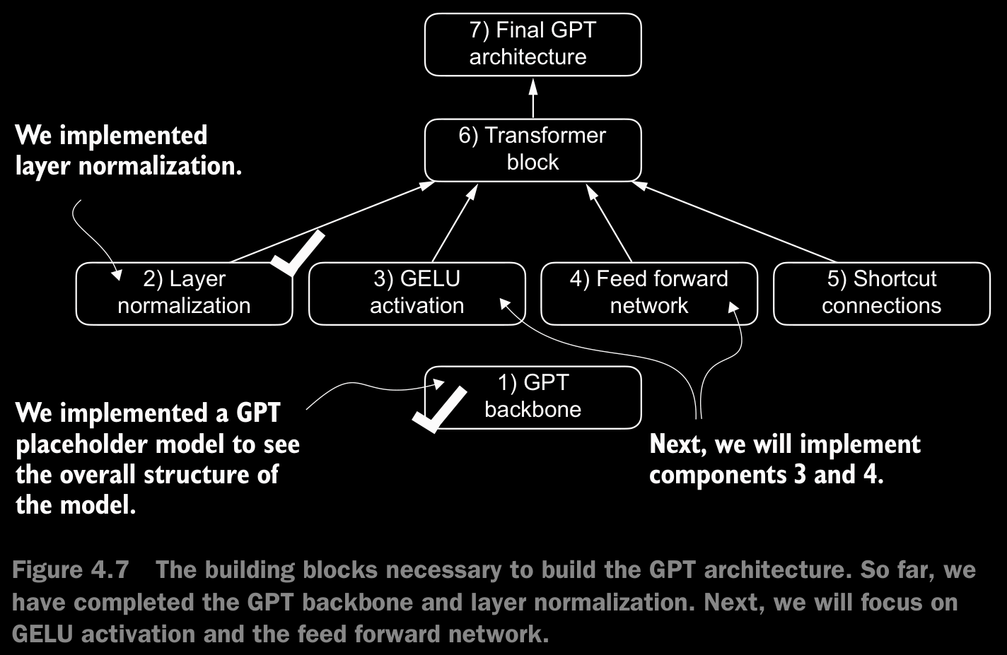Implementing a Feed Forward Network with GELU Activations

• GELU (Gaussian error linear unit) and SwiGLU (Swish-gated linear unit).
• GELU and SwiGLU are more complex and smooth activation functions incorporating Gaussian and sigmoid-gated linear units, respectively. They offer improved performance for deep learning models, unlike the simpler ReLU.
• $GELU(x)=x\cdot \Phi (x)$ where $\Phi (x)$ is the Cummulative Distribution Function of the Standard Gaussian Distribution.
• In practice, it is common to implement a computationally cheaper approximation (the original GPT-2 was also trained with this approx.) which was found via curve fitting.

$$GELU(x)\approx 0.5\cdot x\cdot \left(1+tam\left[\sqrt{\frac{2}{\pi }}\cdot \left(x+0.044715\cdot x^3\right)\right]\right)$$

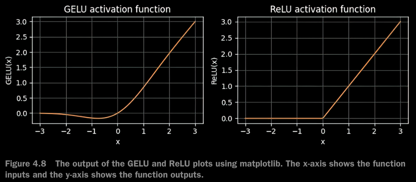
• The smoothness of GELU can lead to better optimization properties during training, as it allows for more nuanced adjustments to the model’s parameters. In contrast, ReLU has a sharp corner at zero, which can sometimes make optimization harder, especially in networks that are very deep or have complex architectures. Moreover, unlike ReLU, which outputs zero for any negative input, GELU allows for a small, non-zero output for negative values. This characteristic means that during the training process, neurons that receive negative input can still contribute to the learning process, albeit to a lesser extent than positive inputs.
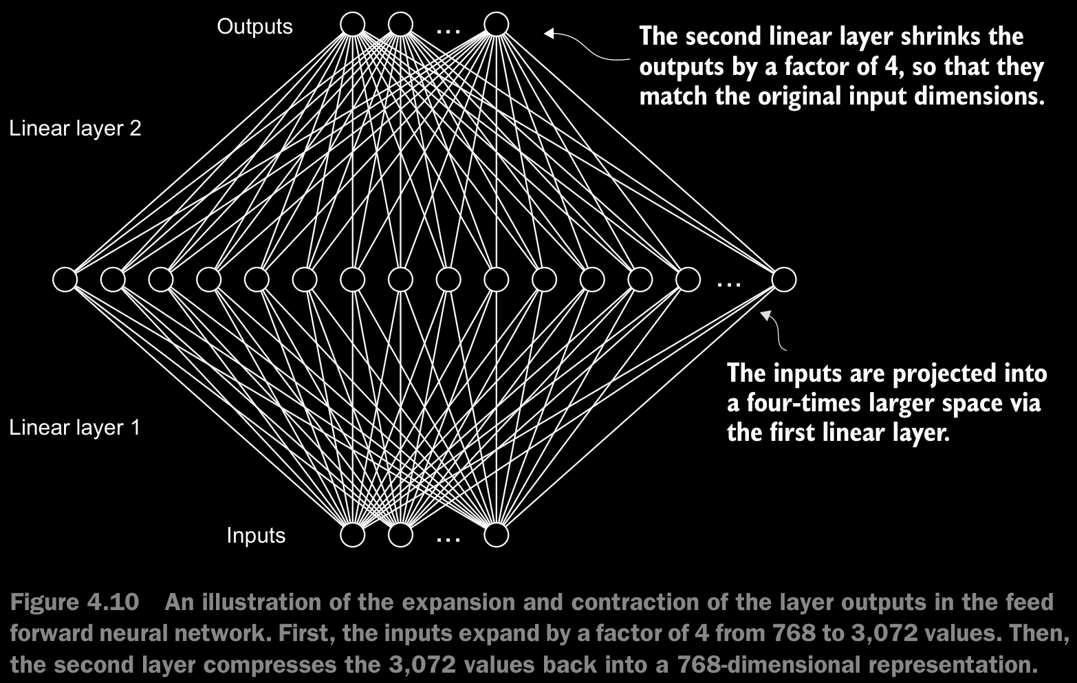
• The FeedForward module plays a crucial role in enhancing the model’s ability to learn from and generalize the data. Although the input and output dimensions of this module are the same, it internally expands the embedding dimension into a higher-dimensional space through the first linear layer, as illustrated in figure 4.10. This expansion is followed by a nonlinear GELU activation and then a contraction back to the original dimension with the second linear transformation. Such a design allows for the exploration of a richer representation space.
• Moreover, the uniformity in input and output dimensions simplifies the architecture by enabling the stacking of multiple layers, as we will do later, without the need to adjust dimensions between them, thus making the model more scalable.

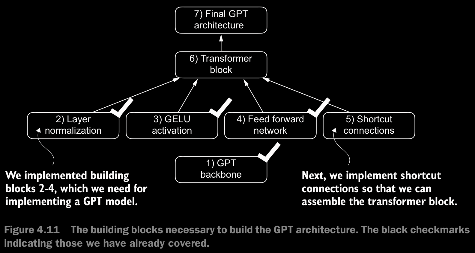
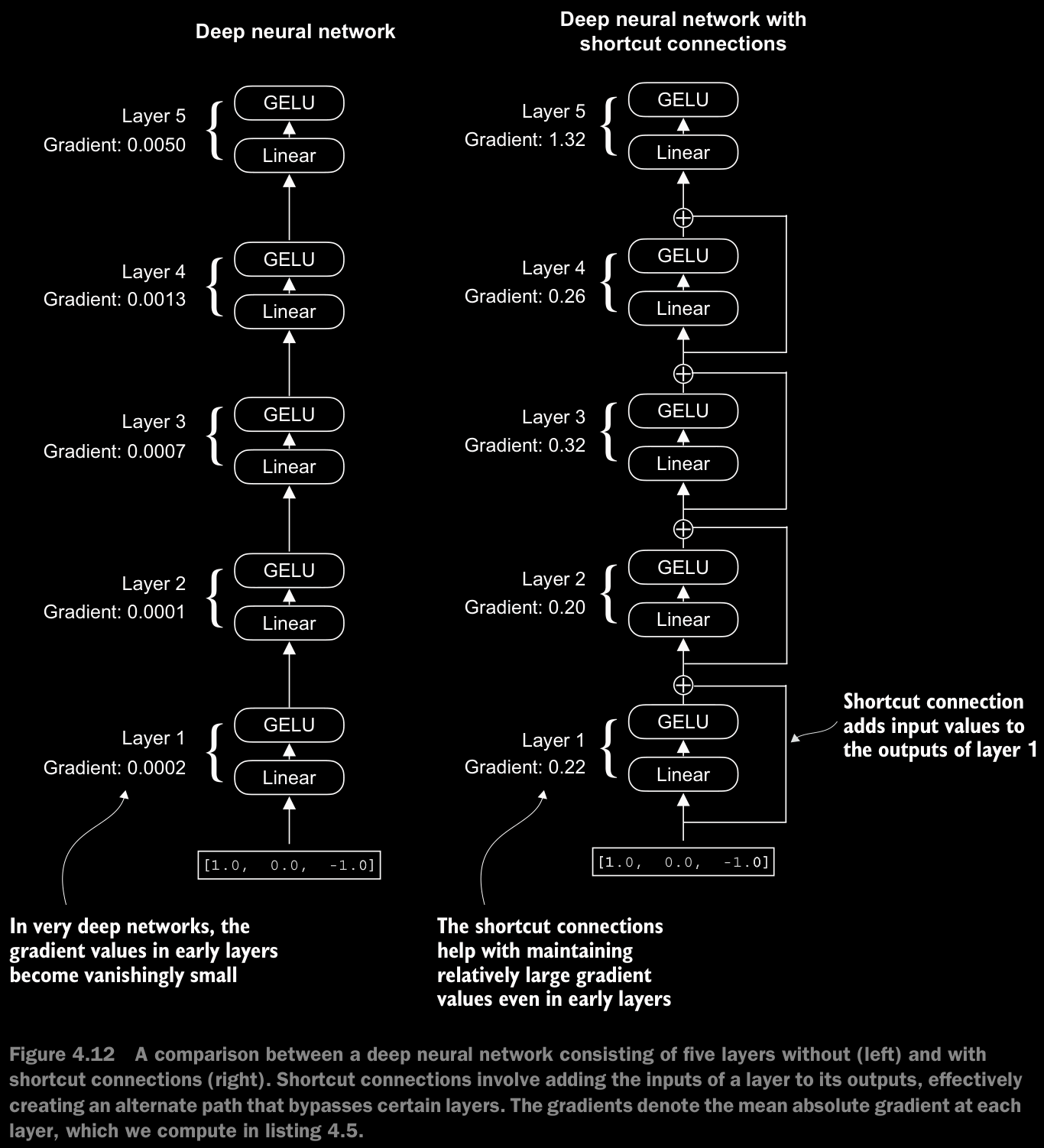
4.4 Adding Shortcut Connections

• a.k.a. skip conntections, residual connections.
• Originally, shortcut connections were proposed for deep networks in computer vision (specifically, in residual networks) to mitigate the challenge of vanishing gradients.

4.5 Connecting Attention and Linear Layers in a Transformer Block

• The idea is that the self-attention mechanism in the multi-head attention block identifies and analyzes relationships between elements in the input sequence. In contrast, the feed forward network modifies the data individually at each position. This combination not only enables a more nuanced understanding and processing of the input but also enhances the model’s overall capacity for handling complex data patterns.
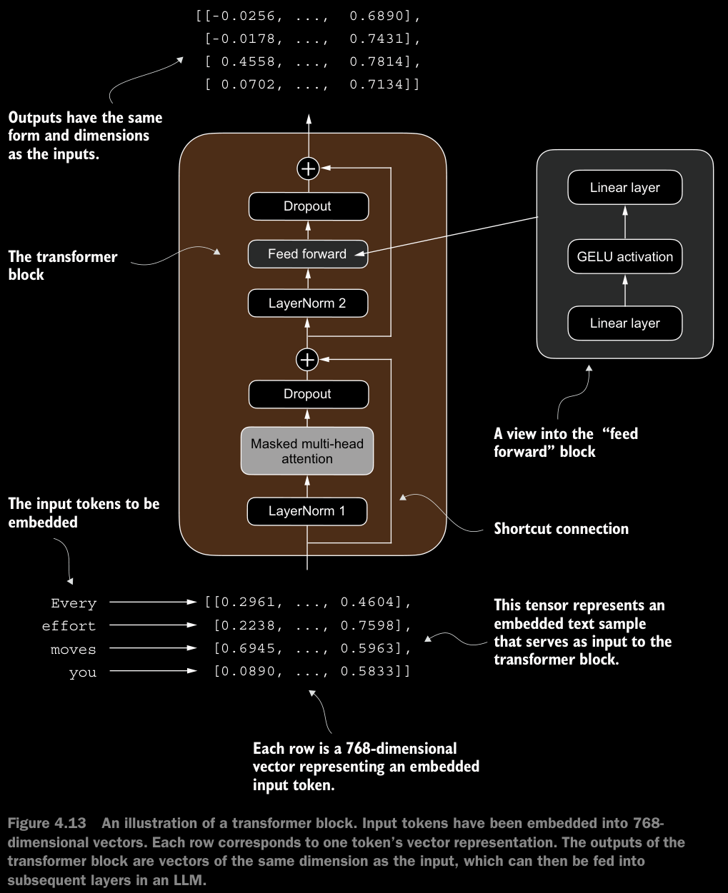
• Layer normalization (LayerNorm) is applied before each of these two components, and dropout is applied after them to regularize the model and prevent overfitting. This is also known as Pre-LayerNorm.
• Older architectures, such as the original transformer model, applied layer normalization after the self-attention and feed forward networks instead, known as Post-LayerNorm, which often leads to worse training dynamics.
• The transformer architecture processes sequences of data without altering their shape throughout the network.
• The preservation of shape throughout the transformer block architecture is not incidental but a crucial aspect of its design. This design enables its effective application across a wide range of sequence-to-sequence tasks, where each output vector directly corresponds to an input vector, maintaining a one-to-one relationship.
• While the physical dimensions of the sequence (length and feature size) remain unchanged as it passes through the transformer block, the content of each output vector is re-encoded to integrate contextual information from across the entire input sequence.

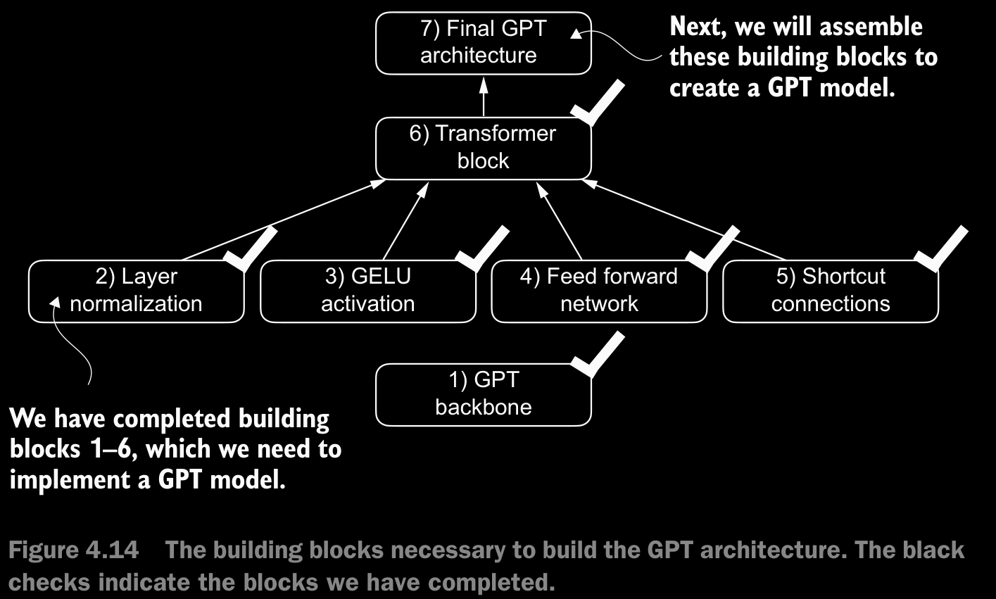
4.6 Coding the GPT Model

• After coding everything out, we a param size of 163009536 instead of getting 124M which is the size we were aiming for. The reason is a concept called weight tying, which was used in the original GPT-2 architecture.
• It means that the original GPT-2 architecture reuses the weights from the token embedding layer in its output layer.
• Since the shape of token embedding layer and output layer, and the num of params here is a lot because of 50257 vocab size, let’s remove the output layer param count from the total GPT-2 model count accg. to the weight tying.
• Weight tying reduces the overall memory footprint and computational complexity of the model. However, using separate token embedding and out put layers results in better training and model performance; hence, we use separate layers in our GPTModel implementation. The same is true for modern LLMs.
• We will implement weight tying concept in chapter 6 when we load pretrained weights from OpenAI.
• The size of the model with 163M params is 621.83 MB assuming each parameter is a 32-bit float taking up 4 bytes of space.

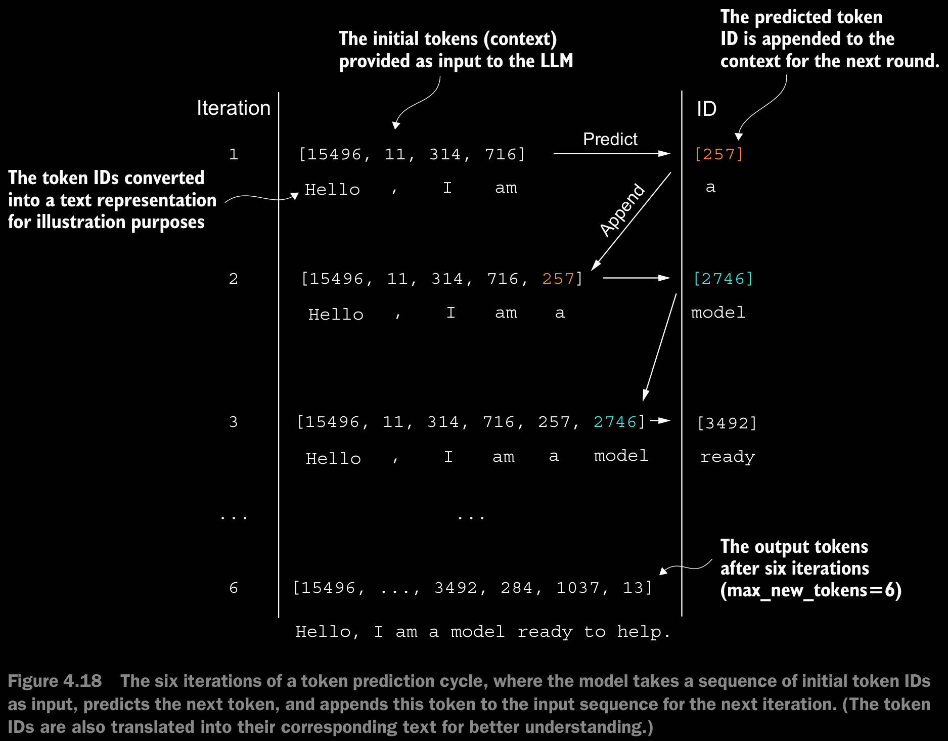
4.7 Generating Text

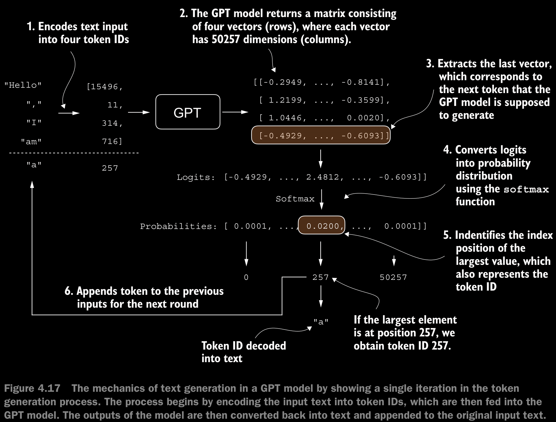
• To code the generate_text_simple function, we use a softmax function to convert the logits into a probability distribution from which we identify the position with the highest value via torch.argmax.
• The softmax function is monotonic, meaning it preserves the order of its inputs when transformed into outputs. So, in practice, the softmax step is redundant since the position with the highest score in the softmax output tensor is the same position in the logit tensor. In other words, we could apply the torch.argmax function to the logits tensor directly and get identical results.
• The code for the conversion to illustrate the full process of transforming logits to probabilities, which can add additional intuition so that the model generates the most likely next token, which is known as greedy decoding.
• When we implement the GPT training code in the next chapter, we will use additional sampling techniques to modify the softmax outputs such that the model doesn’t always select the most likely token. This introduces variability and creativity in the generated text.