Keeping Neural Networks Simple by Minimizing the Description Length of the Weights

0. Abstract

Supervised NNs generalize well if there is much less information in the weights than there is in the output vectors of the training cases.

When a neural network has fewer bits of information in its weights than there are in the output vectors, it suggests that the model is not overly complex and is less likely to overfit to noise in the training data.
Hence, it is necessary to keep the weights small for better generalization which is done through regularization.
The amount of information in a weight can be controlled by adding Gaussian noise. The noise level can be adapted during learning to optimize the trade-off between the expected squared error of the network and the amount of information in the weights.
Provided the output units are linear, the exact derivatives can be computed efficiently without time-consuming Monte Carlo simulations.

A method of computing the derivatives of the expected squared error and of the amount of information in the noisy weights in a network that contains a layer of non-linear hidden units is presented. Provided the output units are linear, the exact derivatives can be computed efficiently without time-consuming Monte Carlo simulations.

1. Introduction

possible ways to limit the information in weights

Limit the number of connections
Divide the connections into subsets, and force the weights within a subset to be identical. If this weight-sharing is based on an analysis of the natual symmetries of the task, it can be very effective (LeNet)
Quantize all the weights in the network so that a probability mass, $p$ , can be assigned to each quantized value. The number of bits in a weight is then $- l o g (p)$ , provided we ignore the cost of defining the quantization. This method unfortunately leads to a difficult search space because the cost of a weight doesn not have a smooth derivative.

1. Limiting the Number of Connections

This approach is the most straightforward but relies on an interesting principle from information theory. When we limit the number of connections, we’re essentially forcing the network to be more selective about what information it stores. Think of it like trying to write a summary of a book - with limited space, you have to be very careful about what information you include.

In a neural network context, this works because:

Each weight can only store a finite amount of information
By reducing the total number of weights, we reduce the network’s total capacity
Thus creating pressure for the network to learn more efficient representations

However, there’s an important caveat here: we’re essentially hoping rather than guaranteeing that the weights won’t store too much information. This is because we don’t have direct control over how much information each individual weight stores.

Weight-sharing is a more sophisticated approach that leverages the inherent structure of the problem being solved. When we force weights within certain subsets to be identical, we’re essentially saying “these connections should respond to the same kinds of patterns.”

Let’s break down why this works:

Natural symmetries: Many tasks have inherent symmetries. For example, in image recognition, a pattern that’s important in one part of the image is often important in other parts too.
Information efficiency: Instead of learning separate weights for similar features, the network uses the same weights multiple times.
LeNet example: In the LeNet architecture, weight-sharing is used in convolutional layers. The same set of weights (filters) slides across the image, looking for the same features in different locations.

The key phrase here is “based on an analysis of the natural symmetries of the task.” This means we’re not arbitrarily sharing weights - we’re doing it based on our understanding of the problem structure. When done this way, it can be very effective because it builds in useful prior knowledge about the problem domain.

3. Weight Quantization

This third approach is particularly interesting from an information theory perspective. Let’s break it down step by step:

The basic idea:

Instead of allowing weights to take any continuous value, we restrict them to a finite set of discrete values
Each possible value has an associated probability $p$
The information content of each weight is measured as $- l o g (p)$ bits

Why this makes sense theoretically:

Information theory tells us that the number of bits needed to encode a value is related to how probable that value is
Less probable values require more bits to encode
This gives us a direct way to measure and control the information content

However, there’s a significant practical challenge here: the cost of a weight does not have a smooth derivative. This is important because:

Gradient based optimization methods require smooth, differentiable cost functions
When we quantize weights, we create discontinuities in the cost function
This makes the optimization process much more difficult

why the derivative isn’t smooth:

When weights are quantized, small changes in the underlying continuous value might not change the quantized value at all
Then suddenly, a tiny change might cause the weight to jump to the next quantized value
This creates a step-like function rather than a smooth one
Gradient-based optimization methods struggle with such discontinuous functions

2. Applying the Minimum Description Length Principle

When fitting models to data, it’s always possible to improve the training data by using a more complex model, but this may make the model worse at fitting new data. So we need some way of deciding when extra complexity in the model is not worth the improvement in the data-fit.

The Minimum Description Length (MDL) Principle

The MDL Principle, introduced by Rissanen, provides an elegant solution to this problem. At its core, the principle states that the optimal model minimizes the sum of two components:

The cost of describing the model itself
The cost of describing the misfit between the model’s predictions and the actual data

In information theory terms, these costs are measured in bits, providing a concrete way to quantify the trade-off between model complexity and accuracy.

Application to Neural Networks

For supervised neural networks with fixed architecture, the MDL principle manifests in two specific costs: Model Description Cost:

Measured in bits required to describe the network weights
Increases with model complexity
Acts as a natural regularizer against overly complex models if used as an optimization target Data Misfit Cost:
Measured in bits needed to describe discrepancies between network outputs and correct answers
Larger errors require more bits to describe
Decreases as the model fits the data better

The Communication Framework

The MDL principle can be understood through a sender-receiver communication scenario: Sender’s Role:

Has access to both input vectors and correct outputs
Trains the neural network
Must communicate:
- Network weights
- Error terms (corrections or adjustments needed for the network’s predictions to match the true outputs exactly. $Δ y$ , elaborated later) for each training case Receiver’s Role:
Only sees input vectors
Receives network weights and error terms
Reconstructs correct outputs by:
- Running inputs through the network
- Adding received error terms

Practical Implications

This framework provides several key insights for model selection: Simple Models:

Low cost for weight description
Higher cost for error description
May be optimal when data is noisy or limited Complex Models:
High cost for weight description
Lower cost for error description
May be optimal with large, clean datasets Finding the Sweet Spot:
The optimal model minimizes total description length
Automatically balances complexity against accuracy
Provides natural regularization

Theoretical Significance

The MDL principle connects to several fundamental concepts in machine learning: Information Theory:

Links model selection to data compression
Provides quantifiable metrics for model evaluation
Grounds intuitive notions of simplicity in mathematical theory Generalization:
Explains why simpler models often generalize better
Provides theoretical foundation for regularization techniques
Helps guide model architecture decisions

Implementation Considerations

When applying MDL in practice: Weight Quantization:

Affects how precisely weights can be communicated
Influences model description cost
Must balance precision against description length Error Encoding:
Requires efficient representation of discrepancies
May use different encoding schemes for different error distributions
Affects overall model evaluation Architecture Selection:
MDL can guide choices about network size and structure
Helps determine when to stop adding complexity
Provides objective criteria for model comparison

Broader Applications

The MDL principle extends beyond neural networks: Model Selection:

Applies to any statistical modeling scenario
Helps choose between competing models
Provides objective complexity measures Regularization:
Justifies common regularization techniques
Suggests new approaches to controlling model complexity
Links to other information-theoretic approaches Understanding Learning:
Provides insights into why certain models work better
Helps explain successful architectural patterns
Guides development of new approaches

3. Coding the Data Misfits

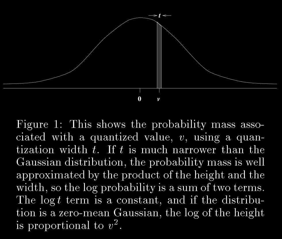
To apply the MDL principle, we need to decide on a coding scheme for the data misfits (differences between the actual outputs predicted by a model and the desired/true outputs) and for the weights.
Clearly, if the data misfits are real numbers, an infinite amount of information is needed to convey them. So, we shall assume that they are very finely quantized, using intervals of fixed width $t$ (which means each number is rounded to the nearest multiple of this interval). We shall also assume that the data misfits are encoded separately for each of the output units.

Coding Theory Basics

Coding theory is concerned with representing data efficiently. A simplified breakdown of relevant concepts:

Information and Bits

Information is often measured in bits (binary digits).
The more uncertain or random something is, the more bits are required to describe it.

Probabilities and Encoding

If you know something is very likely to happen, you can describe it using fewer bits. If it’s unlikely, you need more bits.

Applying Coding Theory to Data Misfits

Probability Distribution

To encode data misfits efficiently, we use a probability distribution $p (Δ y)$ , where $Δ y$ represents the quantized misfit (the difference between predicted and true values).
The coding theorem tells us that if we know the probability distribution of these misfits, we can encode each one using $- lo g_{2} p (Δ y)$ bits.

Gaussian (Normal) Distribution

It’s assumed that the data misfits follow a Gaussian distribution.
This distribution is defined by two parameters:
- Mean (average) Here assumed to be zero (zero-mean).
- Standard deviation $σ_{j}$

Formula for Probability

The probability of a specific misfit $Δ y = d_{j}^{c} - y_{j}^{c}$ (difference between predicted and actual output) is given by:

p (d_{j}^{c} - y_{j}^{c}) = t \frac{1}{2 π σ _{j}} exp [\frac{- ( d _{j}^{c} - y _{j}^{c} ) ^{2}}{2 σ _{j}^{2}}] (1)

- Here, $t$ is the quantization width.
- $d_j^c$ is the desired output for unit $j$ on training case $c$
- $y_j^c$ is the actual output
- $\sigma_j$ is the standard deviation for unit $j$

The standard Gaussian PDF (Probability Density Function) for a random variable $x$ with mean $μ = 0$ , standard deviation $σ$ when continuous is:

PDF (x) = \frac{1}{2 π σ} exp (- \frac{x ^{2}}{2 σ ^{2}})

Description Length

Nats vs Bits

Description length is measured in nats instead of bits here.

1 nat = lo g_{2} (e) bits

Number of nats = - lo g_{e} (p)

Number of bits = - lo g_{2} (p)

Using an optimal code, the description length for a specific misfit is:

- lo g p (d_{j}^{c} - y_{j}^{c}) = - lo g t + lo g 2 π + lo g σ_{j} + \frac{( d _{j}^{c} - y _{j}^{c} ) ^{2}}{2 σ _{j}^{2}} 2) (()

- This formula shows that the description length depends on the quantization width $t$, the standard deviation $\sigma_j$, and the *square of the misfit*.

Minimizing Description Length

To find the value of $σ_{j}$ that minimizes the total description length, we take the derivative of the total description length with respect to $σ_{j}$ and set it to zero:

Total Description Length = c \sum [lo g σ_{j} + \frac{( d _{j}^{c} - y _{j}^{c} ) ^{2}}{2 σ _{j}^{2}}] + constant terms

\frac{\partial}{\partial σ _{j}} c \sum [lo g σ_{j} + \frac{( d _{j}^{c} - y _{j}^{c} ) ^{2}}{2 σ _{j}^{2}}] = 0

c \sum [\frac{1}{σ _{j}} - \frac{( d _{j}^{c} - y _{j}^{c} ) ^{2}}{σ _{j}^{3}}] = 0

Multiply with $σ_{j}^{3}$ on both sides.

c \sum σ_{j}^{2} = c \sum (d_{j}^{c} - y_{j}^{c})^{2}

N σ_{j}^{2} = c \sum (d_{j}^{c} - y_{j}^{c})^{2}

σ_{j} = \frac{1}{N} c \sum (d_{j}^{c} - y_{j}^{c})^{2}

Hence to minimize the total description length over all training cases, the optimal value of $σ_{j}$ is the root mean square (RMS) deviation of the misfits:

σ_{j} = \frac{1}{N} c \sum (d_{j}^{c} - y_{j}^{c})^{2}

- This RMS is essentially the square root of the average squared misfit, which measures the average error magnitude.

Total Cost

Summing over all training cases, the total description length (cost) becomes:

C_{data-misfit} = k N + \frac{N}{2} lo g [\frac{1}{N} c \sum (d_{j}^{c} - y_{j}^{c})^{2}] 3) (()

- Here, $k$ is a constant depending only on $t$.
- This cost function looks similar to the **mean squared error (MSE)** commonly used in regression tasks, showing a *direct connection between minimizing description length and minimizing the MSE*.

Conclusion

The Gaussian assumptions made for the coding of misfits justify using the squared error function in the MDL framework.
By minimizing the description length, we are essentially minimizing the MSE, which supports the MDL principle of seeking the simplest model that explains the data effectively.

Summary

MDL Principle: Prefers simpler models that require fewer bits to describe.
Data Misfits: Differences between actual and predicted outputs are encoded using coding theory.
Quantization: Misfits are quantized to manage infinite precision.
Probability Distribution: Misfits are assumed to follow a Gaussian distribution.
Description Length: Encoding misfits efficiently requires minimizing their description length.
Minimization: Minimizing this length leads to using the mean squared error, aligning with common practices in regression.

4. A Simple Method of Coding the Weights

Similar to data misfits’ encoding, We assume that the weights o fthe trained network are finely quantized and come from a zero-mean Gaussian distribution.
The standard deviation $σ_{w}$ of the Gaussian distribution for weights is fixed. This means that the variability of the weights is predefined and not adjusted during the coding process.
The description length for encoding the weights becomes proportional to the sum of the squares of the weights. This stems from the nature of the Gaussian distribution and how entropy or information content is calculated in this context. Following are the details about it.

Gaussian Distribution and Entropy

The probability density function (PDF) for a Gaussian distribution is given by:

p (x) = \frac{1}{2 π σ ^{2}} exp (- \frac{( x - μ ) ^{2}}{2 σ ^{2}})

Here:

$μ$ is the mean.
$σ^{2}$ is the variance.
$x$ represents the value we are encoding (in this case, the weights).

Entropy of a Gaussian Distribution:

The entropy $H$ of a continuous random variable $X$ with a Gaussian distribution is given by:

H (X) = \frac{1}{2} lo g (2 π e σ^{2})

Entropy represents the average uncertainty or the minimum expected number of bits (or nats, depending on the base of the logarithm) needed to encode a sample from this distribution. The key point here is that entropy (and thus the coding length) depends directly on the variance $σ^{2}$ .

Coding Length and Description Length

In information theory, the description length (or coding length) of a value drawn from a distribution is the negative log-likelihood of that value under the distribution as seen till now.

For a Gaussian-distributed weight $w_{ij}$ , the description length (in nats) can be expressed as the negative log-probability of observing that weight:

- lo g p (w_{ij}) = - lo g (\frac{1}{2 π σ _{w}^{2}} exp (- \frac{w _{ij}^{2}}{2 σ _{w}^{2}}))

This simplifies to:

- lo g p (w_{ij}) = \frac{w _{ij}^{2}}{2 σ _{w}^{2}} + \frac{1}{2} lo g (2 π σ_{w}^{2})

Proportionality to the Sum of Squares

When considering the total description length for all weights $w_{ij}$ in the network, we sum the individual description lengths:

Total description length \propto ij \sum \frac{w _{ij}^{2}}{2 σ _{w}^{2}}

Here, the sum of the squares of the weights $\sum_{ij} w_{ij}^{2}$ becomes the dominant term when focusing on minimizing the description length.

Why the Sum of Squares?

The sum of squares arises because:

The Gaussian distribution places higher probabilities (i.e., shorter coding lengths) on values closer to the mean (zero, in this case).
The quadratic term $\frac{w _{ij}^{2}}{2 σ _{w}^{2}}$ in the exponent reflects the penalty for deviating from the mean, making the coding length quadratic in the deviation.
This quadratic penalty is natural for Gaussian distributions and reflects the fact that larger weights are less probable and thus require more bits (or nats) to encode.

Regularization Perspective

In machine learning, this directly leads to L2 regularization (also known as ridge regression or weight decay), where we penalize the sum of the squares of the weights:

\frac{1}{2 σ _{w}^{2}} ij \sum w_{ij}^{2}

This term acts as a regularizer, encouraging smaller weights and thereby reducing model complexity. Smaller weights correspond to a simpler, more generalizable model.

Total Description Length

The Total Description Length combining Data Misfits’ description length and weights’ description length for all cases ( $c$ ) over all ouput units ( $j$ ) is given by,

C = j \sum \frac{1}{2 σ _{j}^{2}} c \sum (d_{j}^{c} - y_{j}^{c})^{2} + \frac{1}{2 σ _{w}^{2}} ij \sum w_{ij}^{2} 4) (()

This is just the standard “weight-decay” (L2 regularization) method. This weight-decay improves generalization and can therefore be viewed as a vindication of this simple MDL approach in which the standard deviations of the gaussians used for coding the data misfits and the weights are both fixed in advance.

Expansion of Standard Weight Decay

An elaboration/expansion of the standard weight decay approach to make the process more accurate is, where the weight distribution in the trained network is modeled more accurately using a mixture of several Gaussians.

Each Gaussian has its own mean, variance, and mixing proportion, which are adapted during training.

This approach allows for a more refined modeling of the weight distribution and can lead to better generalization, particularly when only a small number of distinct weight values are necessary.

More Flexible Regularization can be done with this approach. Different parts of the network may require different regularization strengths and Multiple Gaussians allow different regularization strengths simultaneously. Each Gaussian component can handle a different “class” of weights and the model can automatically adapt regularization to different network regions.

The mixture model adapts during training through: Learning Phase Adaptation:

Early training: Broader distributions allow exploration
Late training: Distributions narrow as weights stabilize Task-Specific Adaptation:
Simple tasks: Might use fewer Gaussians
Complex tasks: Might utilize more components Layer-Wise Adaptation:
Input layer: Might need precise weights for feature detection
Hidden layers: Could use different distributions for different feature levels
Output layer: Might require another specific distribution type

Despite the improvements, this more elaborate scheme has a serious weakness:

It assumes that all weights are quantized with the same tolerance.
and also assumes that this tolerance is relatively small compared to the standard deviations of the Gaussians modeling the weight distribution.

As a result, this scheme accounts for the probability density of a weight (the height of the Gaussian distribution), but ignores the precision (the width of the distribution). This results in an inefficient use of bits since it doesn’t leverage the full potential of precision variation across different weights as a network is clearly much more economical to describe if some of the weights can be very impercisely described without significantly affecting the predictions of the network.

Summary:

Weight decay is a standard technique that encourages small weights, improving generalization by aligning with MDL principles.
A more sophisticated method involves using a mixture of Gaussians to model weight distributions, potentially improving generalization.
However, this method may inefficiently use bits by not accounting for variations in weight precision.
Future work (MacKay and others) explores how to encode weights more efficiently by considering both their precision and impact on network performance, aiming for a more economical description of the network.

5. Noisy Weights

A standard way of limiting the amount of information in a number is to add zero-mean Gaussian noise. At first sight, a noisy weight seems to be even more expensive to communicate than a precise one since it appears that we need to send a variance as well as a mean, and that we need to decide on a precision for both of these. As we shall see, however, the MDL framework can be adapted to allow very noisy weights to be communicated very cheaply.

Very noisy weights can be communicated cheaply because they require less precision. In information-theoretic terms, if a weight has high variance, its exact value is less critical, and fewer bits are needed to describe it.

The standard approach in training neural networks involves backpropagation:

Start at a specific point in the weight space.
Move this point in the direction that reduces the error function (usually by computing the gradient of the error with respect to the weights). This method focuses on finding a single, precise set of weight values that minimizes the error.

An alternative training method is proposed:

Instead of starting with a single point in the weight space, start with a multivariate Gaussian distribution (multi-dimentional, one for each weight) over weight vectors.
This distribution has both a mean and a variance for each weight.
During training, both the mean and the variance are adjusted to reduce a cost function.
This method captures a cloud of possible weight vectors rather than a single deterministic vector, which provides a probabilistic view of the weights.

The cost function is the expected description length of the weights and of the data misfits.

Variance in this context refers to how spread out the possible values of a weight are, according to its Gaussian distribution.

A high-variance weight implies:
- There is significant uncertainty or flexibility in the value of that weight.
- The weight can vary widely without a precise, fixed value.

These high-variance weights are cheaper to communicate. This is because, In information theory, describing something precisely requires more information (bits). If a weight has a high variance, it means it can be described imprecisely with fewer bits:

The range of acceptable values is broader.
The precision needed to encode the weight is lower.
This reduces the information content required to describe the weight, making it “cheaper” in terms of communication cost (i.e., fewer bits are needed).

5.1 The Expected description Length of the Weights

Posterior Distribution (Q):

The posterior distribution is the updated belief about the weight after observing the data.
It incorporates the information from both the prior distribution and the data (likelihood) through Bayes’ theorem:

Q (w) = \frac{Likelihood(Data | w ) \times P ( w )}{Evidence} ​

After the learning process, the posterior becomes a Gaussian distribution with updated mean and variance:
- Mean $μ_{Q}$ (typically shifted toward the observed data).
- Variance $σ_{Q}^{2}$ (which may become smaller, indicating more certainty about the weight).

We assume that the sender and the receiver have an agreed Gaussian prior distribution, $P$ , for a given weight. After learning, the sender has a Gaussian posterior distribution, $Q$ , for the weight. A method is described for communicating both the weights and the data misfits and show that using this method the number of bits required to communicate the posterior distribution of a weight is equal to the asymmetric divergence (the Kullback-Liebler distance) from $P$ to $Q$ .

🤓 Yashwanth's Notes

Explorer