Identity Mappings in Deep Residual Networks

Original Paper

1. Introduction

2. Analysis of Deep Residual Networks

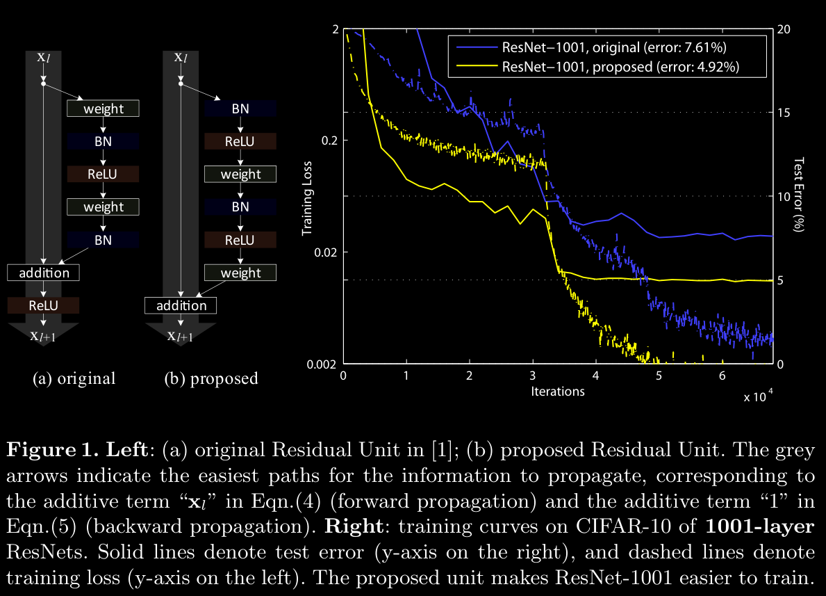
The design of Residual Networks (ResNets) enables deep neural networks to achieve improved performance by introducing modular, stackable “Residual Units” with identity mappings. This design allows information to propagate directly through the network, both forward and backward, without being obstructed by weight layers. Here’s a detailed look at the structure and mathematical properties of ResNets.

a. Residual Units and Basic Equations

Residual Networks are composed of Residual Units that perform specific computations. A Residual Unit in ResNet performs the following operations:

• Primary Equations in a Residual Unit:
  • The output $y_l$ of each Residual Unit at layer $l$ is computed by adding the unit’s input $x_l$ to a residual function $F(x_l,W_l)$, which represents transformations applied to $x_l$ (e.g., convolutional layers). Mathematically, this is given by: $$y_l=h(x_l)+F(x_l,W_l)\text{\hspace{1em}(1)}$$
  • Here, $h(x_l)$ is typically set as an identity mapping, meaning $h(x_l)=x_l$, allowing information to pass directly through each layer.
  • Here $x_l$ is the input feature to the $l$-th Residual Unit. $W_l=\{W_{l,k}{|}_{1\le k\le K}\}$ is a set of weights (and biases) associated with the $l$-th Residual Unit, and $K$ is the number of layers in a Residual Unit ($K$ is 2 or 3 in Original ResNet). $F$ denotes the residual function, e.g., a stack of two 3×3 convolutional layers in Original ResNet. The function $f$ is the operation after element-wise addition, and in Original ResNet $f$ is $ReLU$.
  • The next layer’s input $x_{l+1}$ is then generated by applying a function $f$ to $y_l$: $$x_{l+1}=f(y_l)\text{\hspace{1em}(2)}$$
  • In the original ResNet paper, $f$ is a ReLU activation function, although it can be set as an identity function in specific configurations to simplify information flow.

When $f$ is Set as an Identity Mapping:

If $f$ is also an identity function ($x_{l+1}=y_l$), the equations simplify further:

• By substituting $x_{l+1}$ into $y_l$, we get: $$x_{l+1}=x_l+F(x_l,W_l)\text{\hspace{1em}(3)}$$

This recursive nature allows us to propagate inputs across multiple layers, leading to the Summation Eqn. below.

b. Recursive Formulation of Deep Units

By recursively applying the above transformation across multiple Residual Units, the input $x_L$ at any deeper layer $L$ can be represented as:

$$x_L=x_l+\sum _{i=l}^{L-1}F(x_i,W_i)\text{\hspace{1em}(4)}$$

This recursive formulation reveals two important properties:

1. Residual Connection: The feature $x_L$ of any deep layer $L$ is expressed as the feature $x_l$ of a shallower layer $l$, plus a residual function summed over the intermediate layers. This indicates the network’s residual structure between units $L$ and $l$.
2. Summation of Residual Functions: The feature $x_L$ of a deep layer is the sum of the outputs of all preceding residual functions, plus the initial input $x_0$.

This structure contrasts with standard networks (non-residual), where each feature in deeper layers is a series of matrix-vector multiplications, leading to compounded transformations on the input $x_0$.

c. Backward Propagation in Residual Networks

Residual Networks introduce beneficial properties for backward propagation by preserving gradients effectively across layers, thus reducing the risk of vanishing gradients.

• Gradient Formulation: For a loss function $\mathcal{E}$, the gradient $\frac{\partial \mathcal{E}}{\partial x_l}$ with respect to the input $x_l$ at layer $l$ can be written as: $\frac{\partial \mathcal{E}}{\partial {\mathbf{x}}_l}=\frac{\partial \mathcal{E}}{\partial {\mathbf{x}}_L}\frac{\partial {\mathbf{x}}_L}{\partial {\mathbf{x}}_l}=\frac{\partial \mathcal{E}}{\partial {\mathbf{x}}_L}\left(1+\frac{\partial }{\partial {\mathbf{x}}_l}{\sum }_{i=l}^{L-1}\mathcal{F}({\mathbf{x}}_i,{\mathcal{W}}_i)\right)$

$$\frac{\partial \mathcal{E}}{\partial x_l}=\frac{\partial \mathcal{E}}{\partial x_L}\left(1+\frac{\partial }{\partial x_l}\sum _{i=l}^{L-1}F(x_i,W_i)\right)\text{\hspace{1em}(5)}$$

• Decomposition of Gradient: This equation implies that the gradient can be decomposed into two terms:
  • Direct Term: $\frac{\partial \mathcal{E}}{\partial x_L}$, which propagates back to $x_l$ directly, bypassing any weight layers.
  • Residual Term: $\frac{\partial \mathcal{E}}{\partial x_L}\cdot \frac{\partial }{\partial x_l}{\sum }_{i=l}^{L-1}F(x_i,W_i)$, which propagates through the network’s weight layers.

This decomposition ensures that a part of the gradient flows directly back to any shallower layer $l$, regardless of the transformations in between. This direct propagation reduces the likelihood of gradient vanishing issues, even when weights are arbitrarily small.

d. Implications and Characteristics of Eqn. (4) and Eqn. (5)

These formulations (Eqn. (4) and Eqn. (5)) highlight the unique information propagation characteristics of ResNets:

• Forward Propagation: Signals can propagate through each Residual Unit without being entirely transformed by each layer’s weight.
• Backward Propagation: Gradients flow directly back to shallower units due to the identity connections, ensuring effective gradient flow and reducing vanishing gradient problems.

The foundation of these properties lies in two primary identity mappings:

1. Skip Connection Identity Mapping: $h(x_l)=x_l$.

2. Layer Mapping Identity: When $f$ is an identity mapping, it simplifies information flow further, allowing “clean” pathways without transformations, represented by gray arrows in diagrams.

e. Discussion on Network Design and Practical Impact

The effectiveness of ResNets largely depends on preserving these identity connections to maintain direct information flow across layers:

• Network Depth and Information Flow: These identity mappings allow ResNets to achieve considerable depth by maintaining stable information flow, both forward and backward.
• Regularization of Variance: The identity skip connections also prevent variance from compounding across layers, which is crucial in residual networks where the output of each block is added to the next layer’s input.

This modular design makes ResNets particularly robust to deep architectures, where traditional architectures without residual connections would typically suffer from gradient vanishing or exploding issues.

3. On the Importance of Indentity Skip Connections

a. Modulating the Identity Skip Connection

To understand the significance of this direct path, consider the introduction of a scalar modulation to the identity connection:

$$h(x_l)={\lambda }_l{x}_l$$

This modification gives:

$$x_{l+1}={\lambda }_l{x}_l+F(x_l,W_l)\text{\hspace{1em}(6)}$$

where ${\lambda }_l$ is a scalar specific to each layer $l$ (for simplicity we still assume $f$ is identity). Setting ${\lambda }_l\ne 1$ essentially “breaks” the identity connection, introducing a modulation factor that impacts how much of the input $x_l$ is preserved as the network processes deeper layers.

If we apply this transformation recursively through several layers, we derive an expression for $x_L$ in terms of the original layer $x_l$ as follows:

b. Recursive Formulation of Modulated Skip Connections

To understand the cumulative impact of modulating the identity connection, we can rewrite $x_L$ recursively by expanding each layer:

$$x_L=\left(\prod _{i=l}^{L-1}{\lambda }_i\right)x_l+\sum _{i=l}^{L-1}\left(\prod _{j=i+1}^{L-1}{\lambda }_j\right)F(x_i,W_i)$$

To simplify notation, we introduce a modified residual function $\hat{F}$ that absorbs the scalars $\lambda$, yielding:

$$x_L=\left(\prod _{i=l}^{L-1}{\lambda }_i\right)x_l+\sum _{i=l}^{L-1}\hat{F}(x_i,W_i)\text{\hspace{1em}(7)}$$

This result shows two terms:

• Scalar-modulated term $\left({\prod }_{i=l}^{L-1}{\lambda }_i\right)x_l$, which amplifies or attenuates the original input based on the values of $\lambda$ across layers.
• Modified residual term ${\sum }_{i=l}^{L-1}\hat{F}(x_i,W_i)$, which accumulates the contributions of the residual functions with the scaling factors.

c. Backward Propagation and Gradient Flow Analysis

The key effect of modulating identity connections becomes apparent in backward propagation. For the loss function $\mathcal{E}$, the gradient with respect to the input $x_l$ at layer $l$ is given by:

$$\frac{\partial \mathcal{E}}{\partial x_l}=\frac{\partial \mathcal{E}}{\partial x_L}\left((\prod _{i=l}^{L-1}{\lambda }_i)+\frac{\partial }{\partial x_l}\sum _{i=l}^{L-1}\hat{F}(x_i,W_i)\right)$$

This equation, similar to the unmodulated gradient, is split into two parts:

1. Direct Term: $\frac{\partial \mathcal{E}}{\partial x_L}\left({\prod }_{i=l}^{L-1}{\lambda }_i\right)$, which scales the gradient by the cumulative product of the $\lambda$ factors across layers.
2. Residual Term: $\frac{\partial \mathcal{E}}{\partial x_L}\cdot \frac{\partial }{\partial x_l}{\sum }_{i=l}^{L-1}\hat{F}(x_i,W_i)$, which propagates gradients through the weighted transformations within each layer.

d. Impact of Modulation on Gradient Magnitude

• If ${\lambda }_i>1$ for all layers: The factor ${\prod }_{i=l}^{L-1}{\lambda }_i$ becomes exponentially large as $L$ increases. This amplification can cause excessively large gradients, leading to instability during backpropagation. The model’s updates become erratic, making it difficult to converge to an optimal solution.

• If ${\lambda }_i<1$ for all layers: The factor ${\prod }_{i=l}^{L-1}{\lambda }_i$ diminishes exponentially with depth, leading to a small gradient that effectively vanishes by the time it reaches shallower layers, reducing the flow of information to earlier layers. This forces the gradient to propagate through weight layers only, negating the benefits of the skip connection and making it prone to vanishing gradient problems.

The modulation undermines one of the principal benefits of ResNets: the preservation of gradient strength across layers.

Thus, any deviation from the identity (i.e., $\lambda =1$) causes either an exponential growth or decay in the gradient magnitude, destabilizing the backpropagation process. This is proven by experimental evidence too.

In the above analysis, the original identity skip connection in Eqn.(3) is replaced with a simple scaling $h(x_l)={\lambda }_l{x}_l$. If the skip connection $h(x_l)$ represents more complicated transforms (such as gating and 1×1 convolutions), in Eqn.(8) the first term becomes ${\prod }_{i=l}^{L-1}{h}_i^{\prime }$ where $h^{\prime }$ is the derivative of $h$. This product may also impede information propagation and hamper the training procedure.

3.1 Experiments on Skip Connections

• best practice is to do addition after pre-activations are calculated and then do ReLU on that

3.2 Discussions

a. Direct Pathway of Shortcut Connections

• Shortcut connections are crucial as they offer a direct path for information flow, especially useful in deep networks to mitigate the vanishing gradient problem.
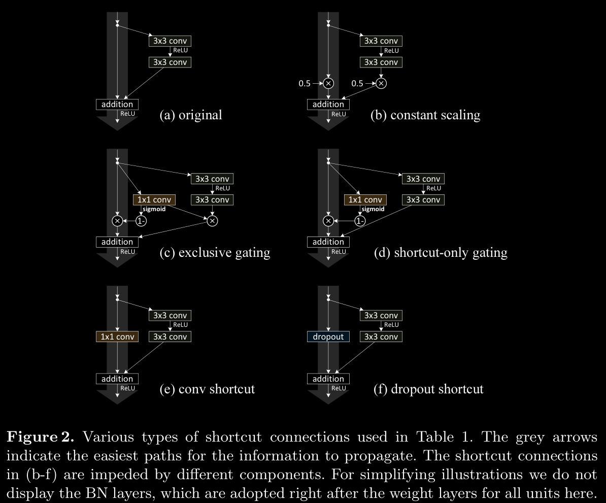
• These connections allow information to skip over several layers, preserving the input signal and its gradient as it propagates through the network. The arrows in Fig. 2 (presumably visual representations of these connections) illustrate how shortcuts act as uninterrupted channels, ensuring information is neither lost nor excessively transformed as it traverses layers.

b. Effects of Multiplicative Manipulations

• Types of Multiplicative Manipulations: Scaling, gating, 1×1 convolutions, and dropout are types of multiplicative operations that can be applied to shortcuts. While each has a distinct function:
  • Scaling and Gating adjust the strength of the signal passing through.
  • 1×1 Convolutions add learnable weights, enhancing the feature transformation capability.
  • Dropout introduces sparsity, preventing certain connections from passing information at all.
• Impact on Propagation: While these operations add flexibility, they can hinder the shortcut’s role as a pure information-preserving channel. Specifically:
  • Scaling and Gating can diminish or overly amplify gradients.
  • 1×1 Convolutions and Dropout alter the shortcut pathway by transforming the signal or even interrupting it, which may prevent consistent propagation.

c. Representational Power of Gated and Convolutional Shortcuts

• Increased Parameters and Complexity: Gating and 1×1 convolutional shortcuts introduce additional parameters, theoretically enhancing the network’s representational power. These shortcuts can express a broader range of transformations than an identity mapping, adapting to complex features and accommodating more diverse transformations.
• Solution Space Coverage: These parameterized shortcuts are flexible enough to cover the solution space of identity shortcuts. In other words, if optimized correctly, these shortcuts could potentially replicate the behavior of identity mappings.

d. Optimization Challenges vs. Representational Abilities

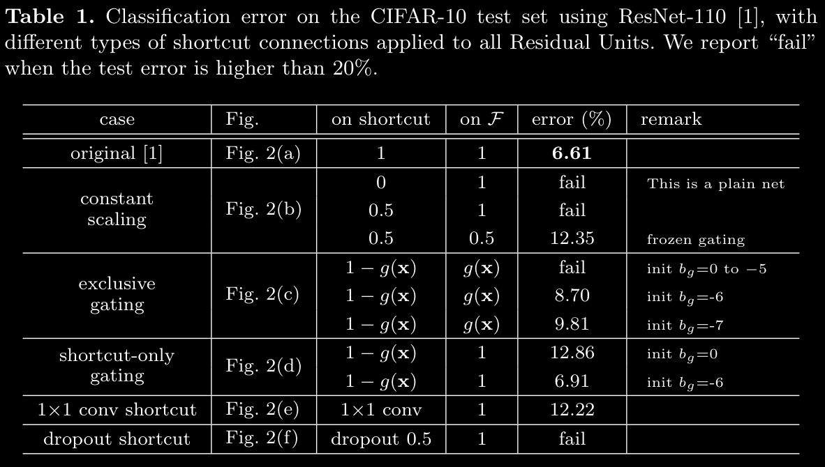
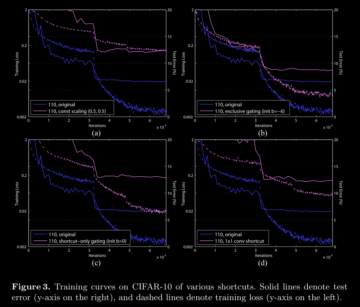
• Higher Training Error in Non-Identity Shortcuts: Empirical findings show that models with gating and 1×1 convolutional shortcuts exhibit higher training errors than those using identity shortcuts. This discrepancy suggests that:
  • The degradation in performance stems from optimization difficulties rather than a limitation in representational power.
  • Despite having sufficient parameters to function like identity shortcuts, the added complexity makes these paths harder to train, as they may lead to increased chances of gradient vanishing or excessive transformation.

4. On the Usage of Activation Functions

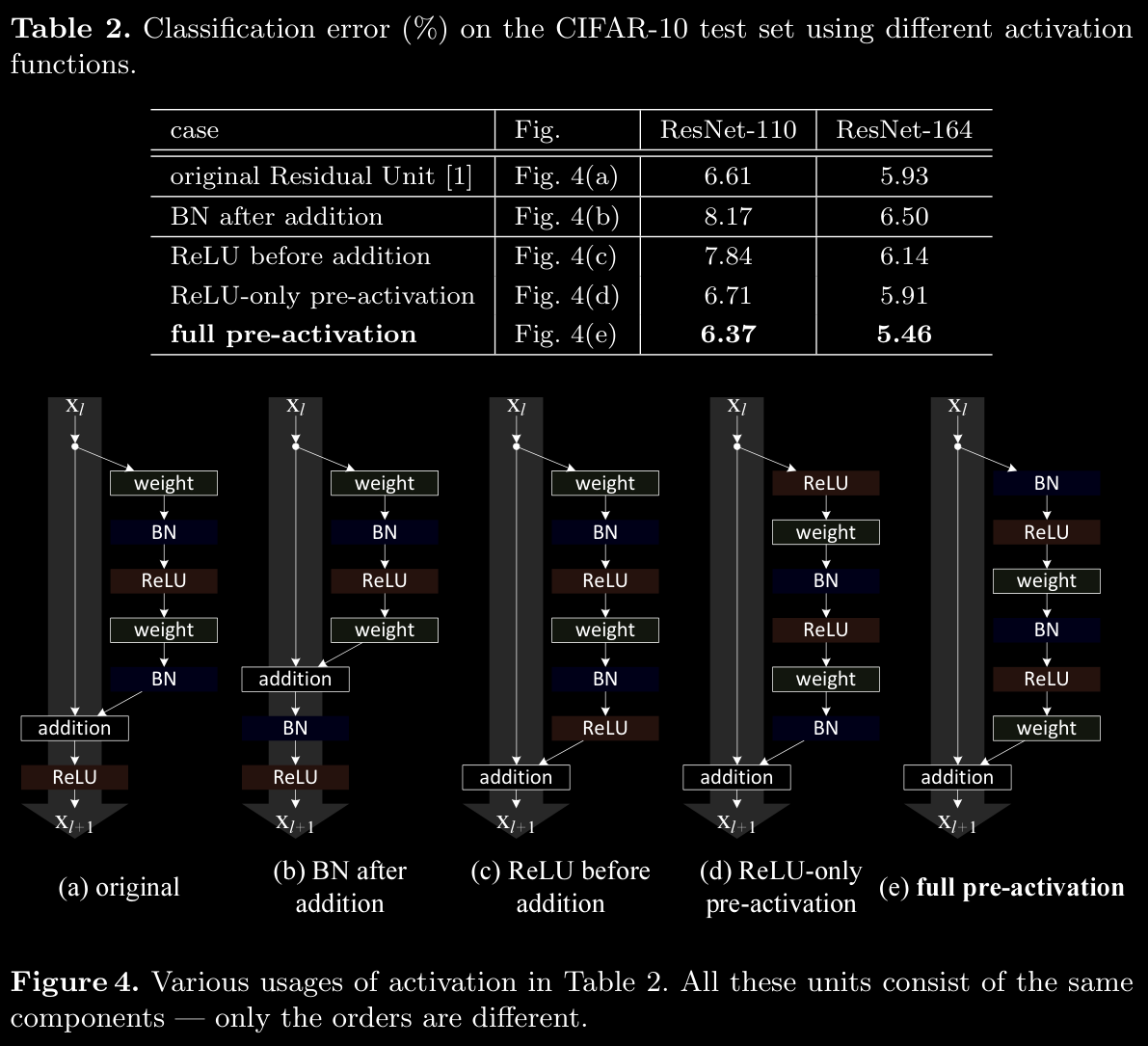
4.1 Experiments on Activations

a. Batch Normalization (BN) After Addition

• Modification: In one setup, Batch Normalization (BN) is applied after the addition operation in residual units.
• Outcome: This configuration causes worse results compared to the baseline (seen in Table 2).
• Explanation:
  • When BN is applied after addition, it disrupts the flow of information in the shortcut paths, making it harder for signals to propagate through the network.
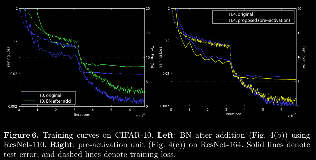
  • This disruption is evident as it results in slower reduction in training loss early in training (illustrated in the left side of Fig. 6).
• Implication: BN after addition is not an optimal configuration as it hinders information flow and gradient stability.

b. ReLU Before Addition

• Modification: Moving ReLU before the addition in the residual connection (Fig. 4(c)).
• Outcome: Leads to worse performance (7.84% on CIFAR-10) than the baseline.
• Explanation:
  • ReLU, applied before addition, outputs only non-negative values, causing the forward-propagated signal to be strictly non-negative and monotonically increasing.
  • A residual function ideally spans the full range of real numbers, $(-\infty ,+\infty )$, but this setup restricts it, limiting the network’s expressiveness.
• Implication: This modification harms the representational capacity of the residual connection, reducing its effectiveness.

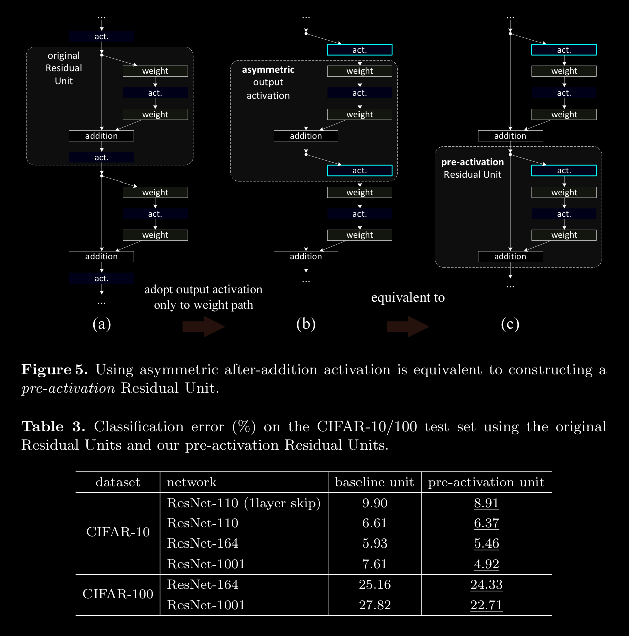
c. Exploring Post-activation vs. Pre-activation

• Original Post-activation Design:

  • In standard ResNet architecture, the activation function (like ReLU) is applied after the addition operation within each residual unit.
  • This design affects both the shortcut path and the residual path in the subsequent unit, making it a post-activation configuration.

• Asymmetric Pre-activation Design:

  • An alternative setup, termed as pre-activation, applies the activation only on the residual path but not on the shortcut.
  • Formulation: $x_{l+1}=x_l+F(\hat{f}(x_l),W_l)$, where $\hat{f}$ denotes the activation function, typically applied before the weight layer (Fig. 5).
  • Result: When using pre-activation, the activation after addition effectively becomes an identity function, making this design advantageous as it ensures cleaner gradient flow during backpropagation.
  • Implication: Pre-activation aligns with the design philosophy of residual networks by maintaining unaltered gradient flow through the shortcut, enhancing network stability.

d. Experiments with ReLU-Only Pre-activation and Full Pre-activation

1. ReLU-Only Pre-activation:
   • In this setup, only ReLU is applied as pre-activation before the residual block (Fig. 4(d)).
   • Performance: Similar to baseline results for ResNet-110 and ResNet-164.
   • Explanation: Applying only ReLU without BN may reduce benefits since BN helps normalize inputs, providing a more stable learning environment. Without BN, ReLU alone might lack the regularization advantages BN typically offers.
2. Full Pre-activation with BN and ReLU:
   • Full pre-activation incorporates both BN and ReLU before the residual blocks (Fig. 4(e)).
   • Performance: Results significantly improve, as evidenced by lower classification error rates across various architectures, including ResNet-1001, with improved training and test error reduction (Table 3).
   • Explanation: BN before ReLU allows each layer to see normalized data with zero mean and unit variance, enhancing learning dynamics.
   • Implication: Full pre-activation leads to improved training stability and performance.

e. Comparative Analysis of Results

• Summary of Results (Table 3):

  • Across all configurations and network depths (ResNet-110, ResNet-164, and ResNet-1001), full pre-activation consistently outperforms the baseline post-activation approach.
  • For CIFAR-10:
    • Pre-activation ResNet-110 shows improvement from 6.61% to 6.37%.
    • Pre-activation ResNet-164 improves from 5.93% to 5.46%.
    • Pre-activation ResNet-1001 sees a large improvement from 7.61% to 4.92%.
  • For CIFAR-100:
    • The pre-activation design also outperforms the baseline, with significant error reduction.
  • Observations:
    • The pre-activation configuration is particularly advantageous in very deep networks (e.g., ResNet-1001), reducing training error by a large margin.

• Training Curves (Fig. 6):

  • BN after addition (left) shows slower convergence and higher training loss, confirming that post-activation setups with BN hinder gradient flow.
  • The pre-activation design (right) results in smoother training curves with lower loss, indicating better optimization.

d. Summary

• Impact of Pre-activation: Moving BN and ReLU before residual layers enhances gradient flow, providing a more stable learning process, especially in very deep networks.
• Optimization and Stability: The pre-activation setup prevents shortcut paths from altering gradient magnitude, allowing information to propagate without significant transformation. This design is crucial for large networks where the risk of gradient vanishing is high.
• Practical Recommendations: For ResNet and similar architectures, full pre-activation (BN + ReLU before residual layers) is a superior configuration that consistently improves performance, especially in deeper networks.
• Design Implication: For modern deep networks, placing BN and activation functions before residual blocks (pre-activation) should be preferred, as it simplifies gradient flow, minimizes representational issues, and enhances the network’s capacity to generalize effectively.

4.2 Analysis

1. Ease of Optimization

• Identity Mapping: Pre-activation simplifies optimization by making the function $f$ an identity mapping. This adjustment allows the signal to flow more freely through the network without the interference of intermediate transformations, notably when layers increase.
• Impact on Deep Layers: In the original design, when ReLU is used as $f$, negative signals are truncated, impeding gradient flow in networks with extensive layers (e.g., 1000+). That means equations Eqn(3), Eqn(5) wont be a good apporximation. This truncation hence affects the optimization, resulting in slow reduction in training error, especially noticeable at the beginning of training (Fig. 1).
• Shorter Networks: For networks with fewer layers (e.g., 164 in Fig. 6), the effect of ReLU truncation is less pronounced. After some training, weights adjust to ensure signals ($y_l$ in Eqn(1)) are more frequently above zero, allowing the model to enter a “healthy” training phase despite initial loss ($x_l$ is always non-negative due to the previous ReLU, so $y_l$ is below zero only when the magnitude of $F$ is very negative). However, with increased layers, truncation by ReLU occurs more frequently, showing the limitations of the original design for ultra-deep networks.

2. Reduced Overfitting via Improved Regularization

• Batch Normalization (BN): Pre-activation introduces BN prior to each weight layer, which has a strong regularization effect. This regularization effect is particularly beneficial in complex models by limiting overfitting.
• Training Loss and Test Error: In the pre-activation model, final training loss is slightly higher than in the baseline; however, the model achieves lower test error, indicating improved generalization.
• Normalization Across Layers: The pre-activation structure ensures that the inputs to all weight layers remain normalized, unlike the original ResNet design where BN occurs only before addition, leaving the merged signal unnormalized. This consistent normalization further enhances model stability and regularization.

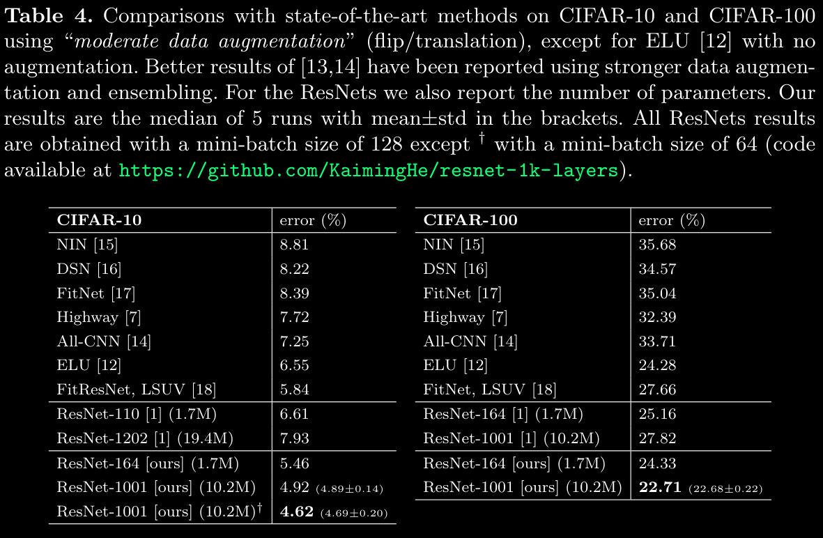
3. Empirical Performance on CIFAR-10 and CIFAR-100

• Competitive Results: The pre-activation ResNet models outperformed the baseline ResNets across both CIFAR-10 and CIFAR-100, with the pre-activation ResNet-1001 achieving the lowest error rate (4.62%) on CIFAR-10 and 22.71% on CIFAR-100 (see Table 4).
• Comparison with Other Models: The pre-activation ResNet consistently performs better than alternative architectures such as FitNet, Highway Networks, and All-CNN on both datasets. This suggests that the pre-activation design brings robustness and efficacy to ResNet models, allowing them to remain competitive with other state-of-the-art methods, especially when combined with moderate data augmentation techniques (flip/translation).

Summary

The adoption of pre-activation in ResNets not only streamlines the optimization process but also introduces a more robust regularization mechanism, resulting in superior performance in deep architectures. By normalizing the signal before each weight layer, the pre-activation ResNet models are both optimized more easily and generalized more effectively. This structural improvement enables deep ResNets to achieve competitive results on challenging datasets like CIFAR-10 and CIFAR-100, illustrating the effectiveness of pre-activation as a design strategy for ultra-deep neural networks.