AlexNet - ImageNet Classification with Deep Convolutional Neural Networks

3.3 Local Response Normalization

• This Normalization is applied to the activations of each kernel after they’ve been through ReLU.
• Normalization is needed for ReLU neurons/kernels as there is no upper bound for these activations. Hence, the values might go very high.
• LRN also acts as a dampener reducing the activation value with it’s main purpose being to increase the sparsity.

1. Background on ReLU Activation and Saturation

The Rectified Linear Unit (ReLU) is a popular activation function for CNNs. Its formula is:

$$\text{ReLU}(x)=\max (0,x)$$

This function has a desirable property: if the input to a ReLU is positive, the output is also positive and simply equal to the input. If the input is zero or negative, the output is zero. This simplicity makes ReLU efficient for backpropagation and helps mitigate the vanishing gradient problem, which can occur in sigmoid or tanh activations. In these other activations, gradients diminish as input values become too large or too small, effectively “saturating” the neuron. However, ReLUs do not saturate in the positive region, so they can support a wider range of input values without requiring input normalization.

2. Why Local Response Normalization is Helpful

Even though ReLUs naturally avoid saturation, a form of local normalization can still enhance generalization in CNNs. Generalization in this context refers to the model’s ability to perform well on unseen data, not just the training set. In this passage, the authors describe a local response normalization (LRN) scheme that improves the model’s ability to generalize by introducing a mechanism similar to lateral inhibition, a phenomenon observed in biological neurons.

3. Notation and Explanation of the Normalization Formula

In this context, let:

• $a_{x,y}^i$: represent the activity (output) of a neuron. This activity is computed by applying the $i$-th kernel at position $(x,y)$ in the image, then passing the result through a ReLU activation.
• $b_{x,y}^i$: represent the normalized activity of the neuron after applying the normalization scheme.

The normalization formula for $b_{x,y}^i$ is:

$$b_{x,y}^i=\frac{a_{x,y}^i}{{\left(k+\alpha {\sum }_{j=\max (0,i-n/2)}^{\min (N-1,i+n/2)}(a_{x,y}^j{)}^2\right)}^{\beta }}$$

Breaking Down the Components:

1. Summation over Adjacent Kernel Maps:

   • The summation is calculated over n adjacent kernels. These kernels apply filters at the same spatial position $(x,y)$ in the feature map. The “neighborhood” of kernels considered for normalization ranges from $i-n/2$ to $i+n/2$, bounded within the total number of kernels $N$ (i.e., $0\le j<N$).
   • This neighboring area defines which neurons “compete” with each other for large activations at each position.

2. Lateral Inhibition Mechanism:

   • By introducing a sum of squared activations of neighboring neurons (from adjacent kernels), the normalization creates a competitive environment. Only neurons with significantly large activations can dominate after normalization, which inhibits other neurons in their “neighborhood” from having high outputs.
   • This competition is biologically inspired by lateral inhibition, where neurons with strong responses suppress the responses of neighboring neurons. This makes the network more selective, helping it focus on stronger, more unique features.

3. Hyperparameters $k$, $\alpha$, $\beta$, and $n$:

   • $k$: A small constant (bias) added to avoid division by zero. Setting $k$ too low could lead to instability.
   • $\alpha$: Controls the influence of the normalization term. A high $\alpha$ would make the network more sensitive to neighboring neuron activations.
   • $\beta$: A scaling exponent applied to the normalization term, controlling how strongly the inhibition affects the final activation.
   • $n$: The number of neighboring kernels (filters) involved in the normalization process.

   The authors mention they used $k=2$, $n=5$, $\alpha =10^{-4}$, and $\beta =0.75$ based on tuning with a validation set.

4. Why This Normalization Helps with Generalization

This response normalization leads to a more sparse activation pattern, where only the most strongly responding neurons in a neighborhood stay active. Sparsity can prevent overfitting by reducing the number of high-magnitude activations, which in turn lowers the model’s capacity to memorize specific details of the training data.

1. Reduces Redundant Responses: Neighboring neurons activated by similar features are suppressed, allowing the network to avoid redundant information and focus on distinct, salient features.

2. Enhances Robustness: The resulting lateral inhibition introduces a type of noise resistance by preventing over-sensitivity to slight feature variations.

5. Comparison with Local Contrast Normalization

The passage briefly compares their response normalization scheme to local contrast normalization (LCN), a technique introduced by Jarrett et al. In LCN, the output of a neuron is adjusted based on the mean and variance of the neuron’s neighborhood, essentially centering the output around zero and emphasizing contrast. The scheme described here, however, does not involve subtracting the mean; thus, it is more accurately described as “brightness normalization”, since it does not re-center the values.

6. Impact on Performance

The authors observe that this normalization reduced the top-1 error rate by 1.4% and the top-5 error rate by 1.2% on their main dataset, highlighting the performance improvement. Furthermore, applying this scheme to the CIFAR-10 dataset with a simple four-layer CNN also demonstrated a significant performance gain, reducing the test error from 13% to 11%.

Summary

Local response normalization introduces a form of lateral inhibition among neighboring neurons, making the network more selective about which neurons respond strongly at each position. This form of normalization can improve the model’s ability to generalize by enhancing feature selectivity and robustness, which prevents over-reliance on specific details of the training data and reduces error rates in classification tasks.

3.4 Overlapping Pooling

Pooling layers in CNNs summarize the outputs of neighboring groups of neurons in the same kernel map. Traditionally, the neighborhoods summarized by adjacent pooling units do not overlap (e.g., [17, 11, 4]). To be more precise, a pooling layer can be thought of as consisting of a grid of pooling units spaced s pixels apart, each summarizing a neighborhood of size z × z centered at the location of the pooling unit. If we set s = z, we obtain traditional local pooling as commonly employed in CNNs. If we set s < z, we obtain overlapping pooling. This is what we use throughout our network, with s = 2 and z = 3. This scheme reduces the top-1 and top-5 error rates by 0.4% and 0.3%, respectively, as compared with the non-overlapping scheme s = 2, z = 2, which produces output of equivalent dimensions. We generally observe during training that models with overlapping pooling find it slightly more difficult to overfit.

Overfitting is not defined over a particular size of dataset. If we have large datasets such as the imagenet, then overfitting could very well be applicable for a large portion of it or a small portion of it. It is simply a phenomenon where a CNN might not learn to extract rich features (more generalizable model), but rather tends to extract features that are only good for classifying certain number of examples in the training set. Excuse my reference to only CNNs, but this argument can be extended to general machine learning.

So, when we have non-overlapping pooling regions, we can see that the spatial information is quickly lost and the network “sees” only the dominant pixel values (winning unit for max pooling for example). This would still provide hierarchical representations, but they would almost always be dominated by the “stronger regions” of an image which then propagate through the network. Effectively, this creates a “bias” in learning which in turn causes an easier potential to overfit.

Let me illustrate this in a different manner. Suppose I take photographs and cover most of it except a bright spot and show them to you, the bright spots all look similar and you learn to identify it. But they could have been from different sources such as a lamp post, headlight of a car, the sun and so on. Unless information from the surrounding is also captured, finer distinguishing cannot be achieved. The overfitting occurs because you almost always see a bright spot and learn to say its a “car” and you turn out to be right since most cars have headlights and you have a lot of photographs of cars having their headlights on, but thats not the only feature you would use to recognise a car and thus would do bad during validation and testing. With overlapping regions, there is less loss of surrounding spatial information. This is why fractional pooling seems even more effective. Note that non-overlapping pooling does not always cause a problem in practice and overlapping pooling regions or fractional pooling only marginally improves results. I had to explain it more dramatically to put forth my point.

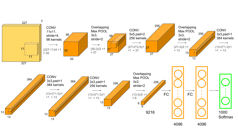
3.5 Overall Architecture

4. Reducing Overfitting

Our neural network architecture has 60 million parameters. Although the 1000 classes of ILSVRC make each training example impose 10 bits of constraint on the mapping from image to label, this turns out to be insufficient to learn so many parameters without considerable overfitting. Below, we describe the two primary ways in which we combat overfitting.

The “10 bits of constraint” refers to the amount of information provided by each training example in the context of classifying images into one of the 1,000 classes in the ILSVRC (ImageNet Large Scale Visual Recognition Challenge) dataset.

Here’s a breakdown of the term:

1. Bits of Information for Classification:

   • In the context of classification, the entropy or information content of a label for a particular class can be calculated as ${\log }_2(C)$, where $C$ is the number of possible classes.
   • For ILSVRC, there are 1,000 classes, so each label provides:
   $${\log }_2(1000)\approx 10\text{ bits}$$
   • This value represents the amount of information needed to specify or “constrain” the label of each image in the dataset, given that the network needs to distinguish between 1,000 possible categories.

2. Implication for Learning Parameters:

   • Each example contributes roughly 10 bits of information about the correct class. However, with 60 million parameters, the model is highly flexible and capable of learning complex mappings but also very susceptible to overfitting.
   • The limited 10-bit constraint per example is therefore insufficient to prevent overfitting on such a large model because each training example constrains only a small fraction of the parameters. Without regularization, the model can memorize training examples rather than generalizing well.

In summary, the “10 bits of constraint” quantifies the information each example provides for classification in a 1,000-class setting, and it highlights that each training example’s information alone is inadequate to fully “constrain” or regularize a model with millions of parameters, thus necessitating additional techniques to combat overfitting.